
2D Turbulence Simulation (SciPy / CuPy / MLX)
Source code: https://github.com/mannetroll/palinstrophy
A Direct Numerical Simulation (DNS) code for 2D homogeneous incompressible turbulence
It supports:
- SciPy / NumPy for CPU runs
- CuPy (optional) for GPU acceleration on CUDA devices (e.g. RTX 3090)
- MLX for GPU acceleration on Apple Silicon via Metal (e.g. M1)
One-liner CPU/SciPy (macOS)
$ curl -LsSf https://astral.sh/uv/install.sh | sh
$ uv cache clean mannetroll-palinstrophy
$ uv run --python 3.13 --with mannetroll-palinstrophy==0.1.5 turbulence
$ uvx --python 3.13 --from mannetroll-palinstrophy==0.1.5 turbulence
One-liner GPU/CuPy (Windows or Linux with CUDA)
$ uv run --python 3.13 --with "mannetroll-palinstrophy[cuda]==0.1.5" turbulence
$ uvx --python 3.13 --from "mannetroll-palinstrophy[cuda]==0.1.5" turbulence
DNS solver
The solver includes:
- PAO-style random-field initialization
- 3/2 de-aliasing in spectral space
- CNAB2 and LS-IMEX-RK3 time integration
- CFL-based adaptive time stepping (Δt updated from the current flow state)
turbulence GUI (PySide6)
Run the turbulence GUI to:
- Displays the flow field as a live image (fast Indexed8 palette rendering)
- Lets you switch displayed variable:
- U, V (velocity components)
- K (kinetic energy)
- Ω (vorticity)
- ψ (stream function)
- Lets you switch colormap (several built-in palettes)
- Lets you change simulation settings on the fly:
- Grid size N
- Initial spectrum peak K0
- Start spectrum KM3 or PAO
- CFL number CFL
- Time stepper CNAB2 or LS-IMEX-RK3
- Max steps / auto-reset limit
- GUI update interval (how often to refresh the display)
- Displays the adapted Reynolds number Re
Keyboard shortcuts
Single-key shortcuts (application-wide) for fast control:
- H: stop
- G: start
- Y: reset
- V: cycle variable
- C: cycle colormap
- N: cycle grid size
- K: cycle K0
- L: cycle CFL
- P: cycle start spectrum
- S: cycle max steps
- U: cycle update interval
Saving / exporting
From the GUI you can:
- Save the current frame as a PNG image
- Dump full-resolution fields to a folder as PGM images:
- u-velocity, v-velocity, kinetic energy, vorticity, stream function
Display scaling
To keep the GUI responsive for large grids, the displayed image is automatically upscaled/downscaled depending on N.
The window is resized accordingly when you change N.
Installation
Using uv
From the project root:
$ uv sync
$ uv run turbulence
$ uv run sim
To make the initial PAO field reproducible, set the PAO seed before launching the GUI or CLI:
$ export SCIPYTURBO_SEED=4895
$ uv run turbulence
Valid seed values are 1 through 5010.
GUI CLI
$ uv run turbulence N K0 Re STEPS CFL BACKEND UPDATE [SPECTRUM [ITERATIONS [METHOD [MOV]]]]
Where:
- N — grid size (defaults to 2048 on CuPy, 1024 on MLX, 512 on SciPy)
- K0 — peak wavenumber of the energy spectrum
- Re — Reynolds number (e.g. 10000)
- STEPS — max steps before reset/stop
- CFL — target CFL number (defaults to 2.0)
- BACKEND — "cpu", "gpu" (CUDA), "mlx" (Apple Silicon), or "auto"
- UPDATE — DNS steps per GUI timer update (defaults to 2)
- SPECTRUM — "KM3" or "PAO" (optional, defaults to "KM3")
- ITERATIONS — total iterations before the GUI quits; if supplied, put SPECTRUM before it
- METHOD — "CNAB2" or "LS_IMEX_RK3" (optional, defaults to "LS_IMEX_RK3")
- MOV — 1 to save movie frames, or "MOV" to read the MOV environment variable
For example, to run KM3 and quit after 100 iterations:
$ uv run turbulence 512 15 10000 1E5 0.1 auto 10 KM3 100
To use LS-IMEX-RK3 and enable movie frames:
$ uv run turbulence 512 15 10000 1E5 0.1 auto 10 KM3 100 LS_IMEX_RK3 1
Solver CLI
$ uv run sim N Re K0 STEPS CFL BACKEND UPDATE [SPECTRUM [METHOD]]
Where:
- N — grid size (e.g. 256, 512)
- Re — Reynolds number (e.g. 10000)
- K0 — peak wavenumber of the energy spectrum
- STEPS — number of time steps
- CFL — target CFL number (e.g. 0.75)
- BACKEND — "cpu", "gpu" (CUDA), "mlx" (Apple Silicon), or "auto"
- UPDATE — print/update cadence in DNS steps
- SPECTRUM — "KM3" or "PAO" (optional, defaults to "KM3")
- METHOD — "CNAB2", "LS_IMEX_RK3", or "CHECK" (optional, defaults to "CNAB2")
Examples:
# CPU run (SciPy with 4 workers)
$ uv run sim 256 10000 10 1001 0.75 cpu 100 KM3

# CPU run with the original PAO start spectrum
$ uv run sim 256 10000 10 1001 0.75 cpu 100 PAO

# CPU run with PAO and status output every 10 steps
$ uv run sim 256 10000 10 1001 0.75 cpu 10 PAO

# CPU run with the default CNAB2 time stepper
$ uv run sim 256 10000 10 1001 0.1 cpu 100 KM3 CNAB2

# CPU run with the low-storage IMEX RK3 time stepper
$ uv run sim 256 10000 10 1001 0.1 cpu 100 KM3 LS_IMEX_RK3

# Compare CNAB2 and LS_IMEX_RK3 final fields from the same initial condition
$ uv run sim 128 10000 10 200 0.05 cpu 50 KM3 CHECK
CHECK runs CNAB2 and LS_IMEX_RK3 from the same PAO seed, then reports
relative L2/Linf differences for the final spectral vorticity and velocity
fields plus energy and eddy-turnover-time differences. Use a small CFL when
checking method agreement; the methods are not bitwise identical, but the
field differences should shrink as the timestep is reduced.
# Apple Silicon GPU run (MLX / Metal)
$ uv run sim 1024 10000 10 1001 0.75 mlx 100 KM3

# Auto-select backend (CuPy if CUDA is available, else MLX, else SciPy)
$ uv run sim 256 10000 10 1001 0.75 auto 100 KM3
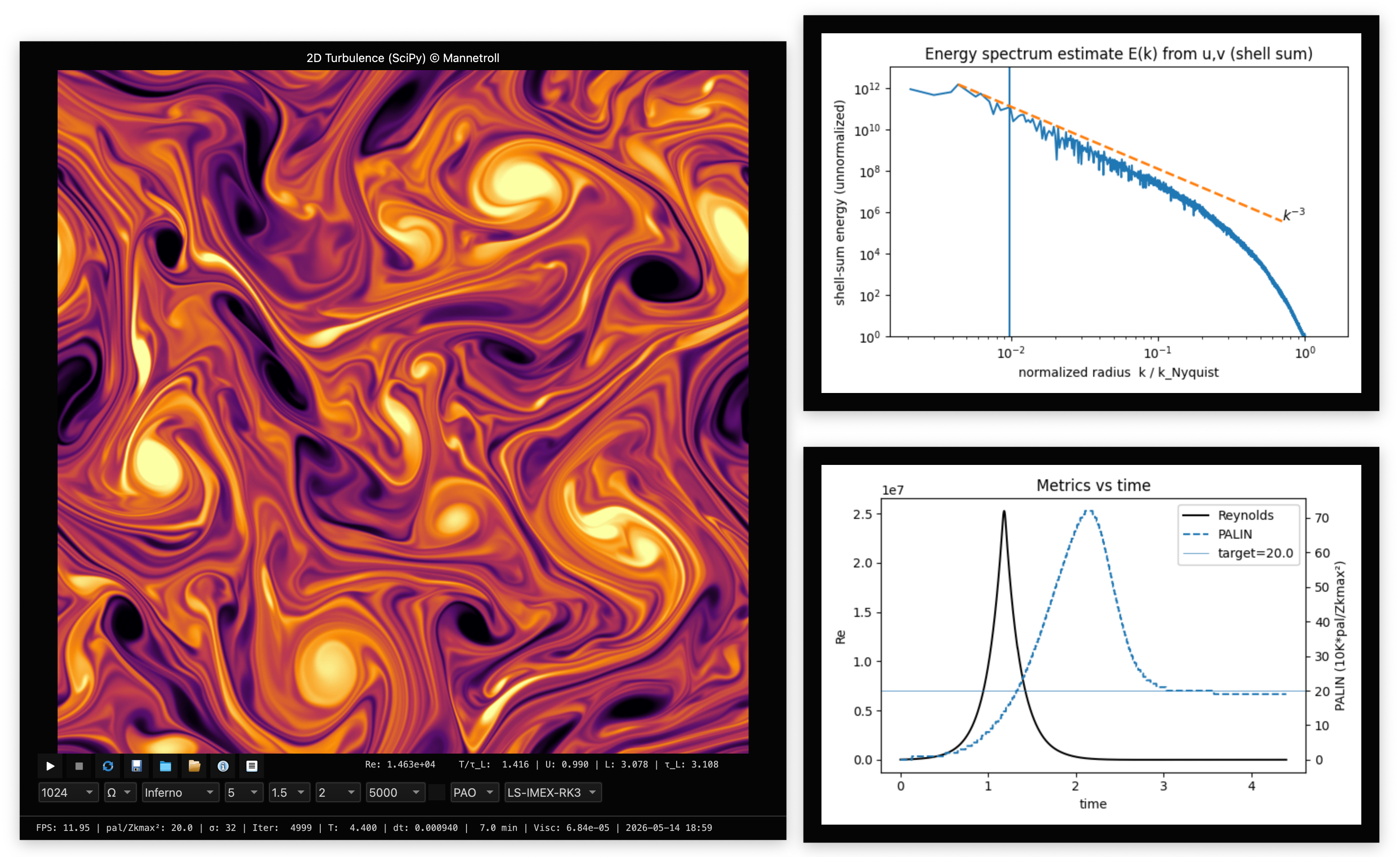
The DNS with SciPy (1024 x 1024)
Enabling GPU with CuPy (CUDA 13)
On a CUDA machine (e.g. RTX 3090):
Download: https://developer.nvidia.com/cuda-downloads
-
Check that the driver/CUDA are available:
$ nvidia-smi -
Install CuPy into the uv environment:
$ uv sync --extra cuda $ uv run turbulence $ uv run sim -
Verify that CuPy sees the GPU:
$ uv run python -c "import cupy as cp; x = cp.arange(5); print(x, x.device)" -
Run in GPU mode:
$ uv run python -m palinstrophy.turbo_simulator 256 10000 10 1001 0.75 gpu 100 KM3
Or let the backend auto-detect:
$ uv run python -m palinstrophy.turbo_simulator 256 10000 10 1001 0.75 auto 100 PAO
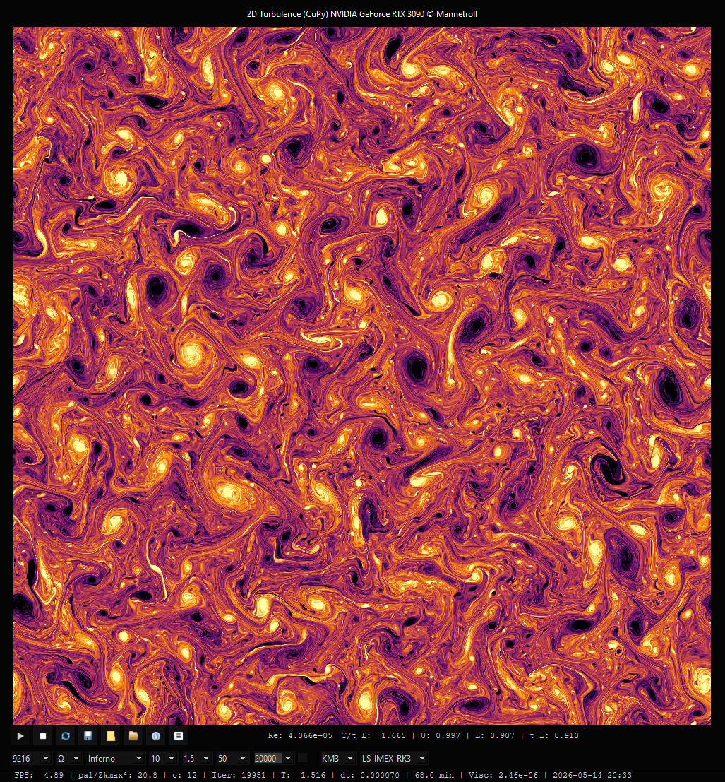
The DNS with CuPy (9216 x 9216) Dedicated GPU memory 20GB of 24GB
Enabling GPU with MLX (Apple Silicon)
MLX is installed automatically by uv sync on Apple Silicon — it is declared with
the marker sys_platform == 'darwin' and platform_machine == 'arm64', so it is
skipped on every other platform. Nothing else is required; Metal ships with macOS.
-
Verify that MLX sees the GPU:
$ uv run python -c "import mlx.core as mx; print(mx.device_info()['device_name'])" -
Run in MLX mode:
$ uv run sim 1024 10000 10 1001 0.75 mlx 100 KM3
Or let the backend auto-detect (CuPy first, then MLX, then SciPy):
$ uv run sim 1024 10000 10 1001 0.75 auto 100 KM3
Measured speedup (Apple M1 Max, CNAB2, KM3, 201 steps)
| N | SciPy FPS | MLX FPS | Speedup |
|---|---|---|---|
| 256 | 752.7 | 1267.0 | 1.7x |
| 512 | 197.8 | 595.8 | 3.0x |
| 1024 | 65.8 | 258.5 | 3.9x |
| 2048 | 13.8 | 68.2 | 4.9x |
The advantage grows with grid size, as the GPU gets enough work to hide launch overhead.
Grid-size limit: keep 3N/2 at or below 4096
MLX's Metal FFT has a fast single-kernel path for transform lengths up to 4096.
Past that it falls back to a path roughly 40x slower — measured on an M1 Max, an
rfft2 of 8 planes takes 17.7 ms at size 4096 and 721 ms at size 4104.
This solver transforms the 3/2 de-aliasing grid, so the transform length is 3N/2
and the usable limit is N <= 2730. In practice:
| N | 3/2 grid | MLX path |
|---|---|---|
| 2048 | 3072 | fast |
| 2560 | 3840 | fast |
| 3072 | 4608 | slow — use cpu instead |
The solver prints a warning when you cross the threshold. Above it the SciPy backend is the faster choice.
Notes on the MLX backend
MLX differs from NumPy and CuPy in ways that shaped the port:
- Slices are copies, not views. The
out=buffer reuse that the SciPy and CuPy paths rely on cannot work, so the MLX paths are written functionally and let MLX fuse the chain itself. - No float64 on Metal. The float64 reductions (
flow_eddy_metrics, the energy spectrum) form their float32 inputs on-device and reduce on the host. Unified memory makes that handoff a view rather than a copy. - Lazy evaluation. Each step ends with an explicit
mx.evalso the graph stays bounded; memory is flat at 230 MiB over 600 steps at N=1024. - Complex-by-real division squares the divisor. MLX evaluates
complex / realas a full complex quotient, so a regulariser like1e-30underflows float32 to zero and yields NaN. Those sites scale by the reciprocal instead.
MLX results track the SciPy reference to float32 precision: relative L2 differences of ~1e-5 after 50 steps, and bulk statistics (energy, eddy-turnover time) agreeing to ~1e-7. The fields diverge slowly with step count, as expected for a chaotic flow integrated in single precision.
Profiling
cProfile (CPU)
$ python -m cProfile -o turbo_simulator.prof -m palinstrophy.turbo_simulator 256 10000 10 201 0.75 cpu 100 KM3
Inspect the results:
$ python -m pstats turbo_simulator.prof
# inside pstats:
turbo_simulator.prof% sort time
turbo_simulator.prof% stats 20
Viewing a cProfile report with SnakeViz
Install SnakeViz:
$ uv pip install snakeviz
Visualize the profile:
$ snakeviz turbo_simulator.prof
Scalene HTML report for the solver CLI
Install Scalene:
$ uv pip install "scalene==1.5.55"
Run the solver and generate Scalene's interactive report:
$ scalene -m palinstrophy.turbo_simulator 256 10000 10 201 0.75 cpu 100 KM3
Scalene terminal report
For a terminal-only summary:
$ scalene --cli --cpu -m palinstrophy.turbo_simulator 512 10000 10 201 0.75 cpu 100 KM3
$ scalene --cli --cpu -m palinstrophy.turbo_main 512 15 10000 1E5 0.1 auto 10 KM3 201
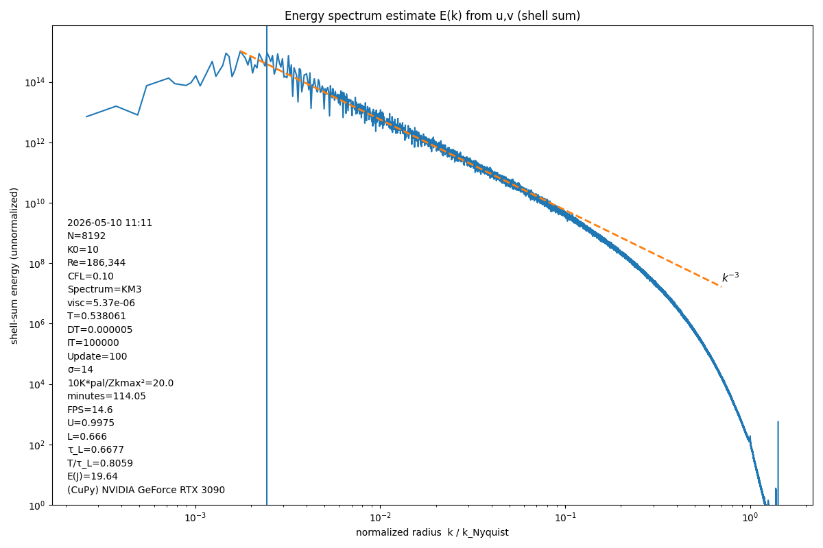
The power spectrum of the energy field
The radially averaged (isotropic) 2D FFT energy spectrum E(k) computed from the velocity fields u and v on log–log axes.
The x-axis is the normalized radial wavenumber (k/k_Nyquist), and the y-axis is the shell-summed spectral energy ∑(|û(k)|² + |v̂(k)|²) accumulated within radial wavenumber bins (DC removed and excluded).
A dashed reference slope k⁻³ is drawn (anchored at the spectral peak) to compare against the expected 2D enstrophy-cascade inertial-range power-law behavior.
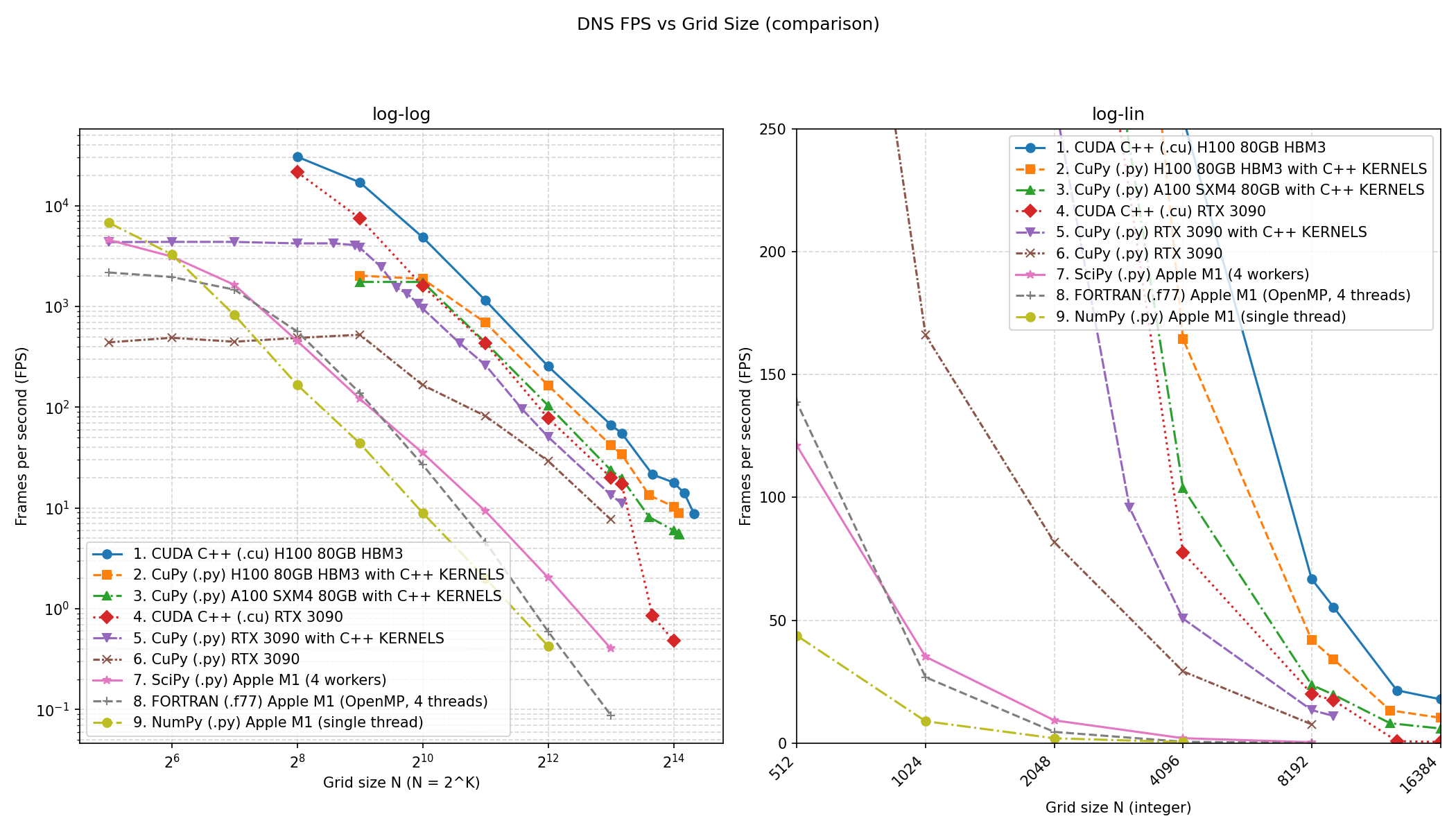
FPS Comparison Plot (DNS FPS vs Grid Size and Code)
Code bases compared
- CUDA C++ (
.cu) — RTX 3090 - CuPy (Python) + custom C++ kernels (
.py+ C++ kernels) — RTX 3090 - CuPy (Python) (
.py) — RTX 3090 - FORTRAN (
.f77) — Apple M1 (OpenMP, 4 threads) - NumPy (Python) (
.py) — Apple M1 (single thread) - SciPy (Python) (
.py) — Apple M1 (4 workers)
NetCDF Restart
Every time you save a case (PGM dump) from the GUI, one NetCDF restart file is written alongside the image files:
| File | Contents |
|---|---|
restart.nc |
Scalar metadata plus spectral fields needed to resume the run |
The complex spectral arrays are stored portably as separate float32 real and imaginary variables:
| Variables | Contents |
|---|---|
uc_real, uc_imag |
Spectral velocity uc — shape (NZ, NK, 3) |
om2_real, om2_imag |
Spectral vorticity om2 — shape (NZ, NX_half) |
fnm1_real, fnm1_imag |
Nonlinear history term fnm1 — shape (NZ, NX_half) |
Scalar metadata is stored as NetCDF attributes: format_version, Nbase, Re, K0, start_spectrum, visc, cflnum, seed_init, t, dt, cn, cnm1, and it.
Loading a restart
Click the folder icon (Load button) in the GUI toolbar. A directory picker opens; select any saved case folder that contains restart.nc. The solver re-initialises with the exact grid size and parameters from the snapshot, restores all spectral arrays, and resumes time-stepping from the saved iteration and simulation time — no random re-initialisation.
This lets you:
- Continue a long run interrupted by a machine restart or out-of-memory event
- Switch backend (CPU ↔ GPU) between runs
- Branch from the same flow snapshot at different Reynolds numbers or CFL values
License
Copyright © 2026 mannetroll
1 maintainer

Release files for mannetroll-palinstrophy 0.1.5
For a detailed explanation of source distributions (sdists) and built distributions (wheels), please see the package formats documentation.
Source distribution (sdist)
| File | Size | Uploaded | |
|---|---|---|---|
| mannetroll_palinstrophy-0.1.5.tar.gz | 327.2 kB | Details |
Built distribution (wheel)
| File | Interpreter | ABI | Platform | Reset |
|---|---|---|---|---|
| mannetroll_palinstrophy-0.1.5-py3-none-any.whl | Python 3 | none | any | Details |
Total release size: 659.2 kB
Release files / mannetroll_palinstrophy-0.1.5.tar.gz
| Download URL | mannetroll_palinstrophy-0.1.5.tar.gz |
|---|---|
| Size | 327.2 kB |
| Tags | Source |
|
SHA-256 checksum How to use checksums |
9b1674bf2047326dc2ff9c428317f867befa85451e77ef70403226cf2279bc0e
|
|
BLAKE2b-256 checksum How to use checksums |
98310fe6dcb5eaec1a56aff958ae7333e4bd66ca67b1c0b9d29d763aa6370cd8
|
| Upload date | |
|
Uploaded using Trusted Publishing? What is trusted publishing? |
No |
| Uploaded via |
twine/6.2.0 CPython/3.13.11
|
Release files / mannetroll_palinstrophy-0.1.5-py3-none-any.whl
| Download URL | mannetroll_palinstrophy-0.1.5-py3-none-any.whl |
|---|---|
| Size | 332.0 kB |
| Tags | Python 3 |
|
SHA-256 checksum How to use checksums |
f491072a918311c03b043c22ddb99ff45a736e6c5f1e4d4bcd49b52fc3afa97a
|
|
BLAKE2b-256 checksum How to use checksums |
b795940975e8ca80ec005da276cf052eb993c675a440eb9a3d9429113c75d304
|
| Upload date | |
|
Uploaded using Trusted Publishing? What is trusted publishing? |
No |
| Uploaded via |
twine/6.2.0 CPython/3.13.11
|














