
Machine Learning Research Wizard

Project description

MLWiz
Machine Learning Research Wizard — reproducible experiments from YAML (model selection + risk assessment) for vectors, images, time-series, and graphs.





🔗 Quick Links
- 📘 Docs: https://mlwiz.readthedocs.io/en/stable/
- 🧪 Tutorial (recommended): https://mlwiz.readthedocs.io/en/stable/tutorial.html
- 📦 PyPI: https://pypi.org/project/mlwiz/
- 📝 Changelog:
CHANGELOG.md - 🤝 Contributing:
CONTRIBUTING.md
✨ What It Does
MLWiz helps you run end-to-end research experiments with minimal boilerplate:
- 🧱 Build/prepare datasets and generate splits (hold-out or nested CV)
- 🎛️ Expand a hyperparameter search space (grid, random, or Bayesian search)
- ⚡ Run model selection + risk assessment in parallel with Ray (CPU/GPU or cluster)
- 📈 Log dashboard-ready metric histories and checkpoints in a consistent folder structure
- 🐍 Export every dashboard plot as reproducible Matplotlib +
tueplotsPython code
Inspired by (and a generalized version of) PyDGN.
✅ Key Features
| Area | What you get |
|---|---|
| Research Oriented Framework | Anything is customizable, easy prototyping of models and setups |
| Reproducibility | Ensure your results are reproducible across multiple runs |
| Automatic Split Generation | Dataset preparation + .splits generation for hold-out / (nested) CV |
| Automatic and Robust Evaluation | Nested model selection (inner folds) + risk assessment (outer folds) |
| Parallelism | Ray-based execution across CPU/GPU (or a Ray cluster) |
| Visualization Dashboard | Explore experiment progress, metric histories, configurations, and model graphs, then export plots as publication-styled Python code |
🚀 Getting Started
📦 Installation
MLWiz supports Python 3.10+.
Create a uv-managed project and add MLWiz:
uv init my-ml-project
cd my-ml-project
uv add mlwiz
If your project already has a pyproject.toml, run only uv add mlwiz from
its root. For GPU or graph workloads, configure PyTorch and PyG following their
official installation instructions before adding MLWiz.
⚡ Quickstart
| Step | Command | Notes |
|---|---|---|
| 1) Prepare dataset + splits | mlwiz-data --config-file examples/DATA_CONFIGS/config_MNIST.yml |
Creates processed data + a .splits file |
| 2) Run an experiment (grid search) | mlwiz-exp --config-file examples/MODEL_CONFIGS/config_MLP.yml |
Add --debug to run sequentially and print logs |
| 3) Inspect results | cat RESULTS/mlp_MNIST/MODEL_ASSESSMENT/assessment_results.json |
Aggregated results live under RESULTS/ |
| 4) Explore in MLWiz Dashboard | mlwiz-dashboard --logdir RESULTS |
Browse model-selection configs and final-run metric histories |
| 5) Stop a running experiment | Press Ctrl-C |
📊 Visualization Dashboard
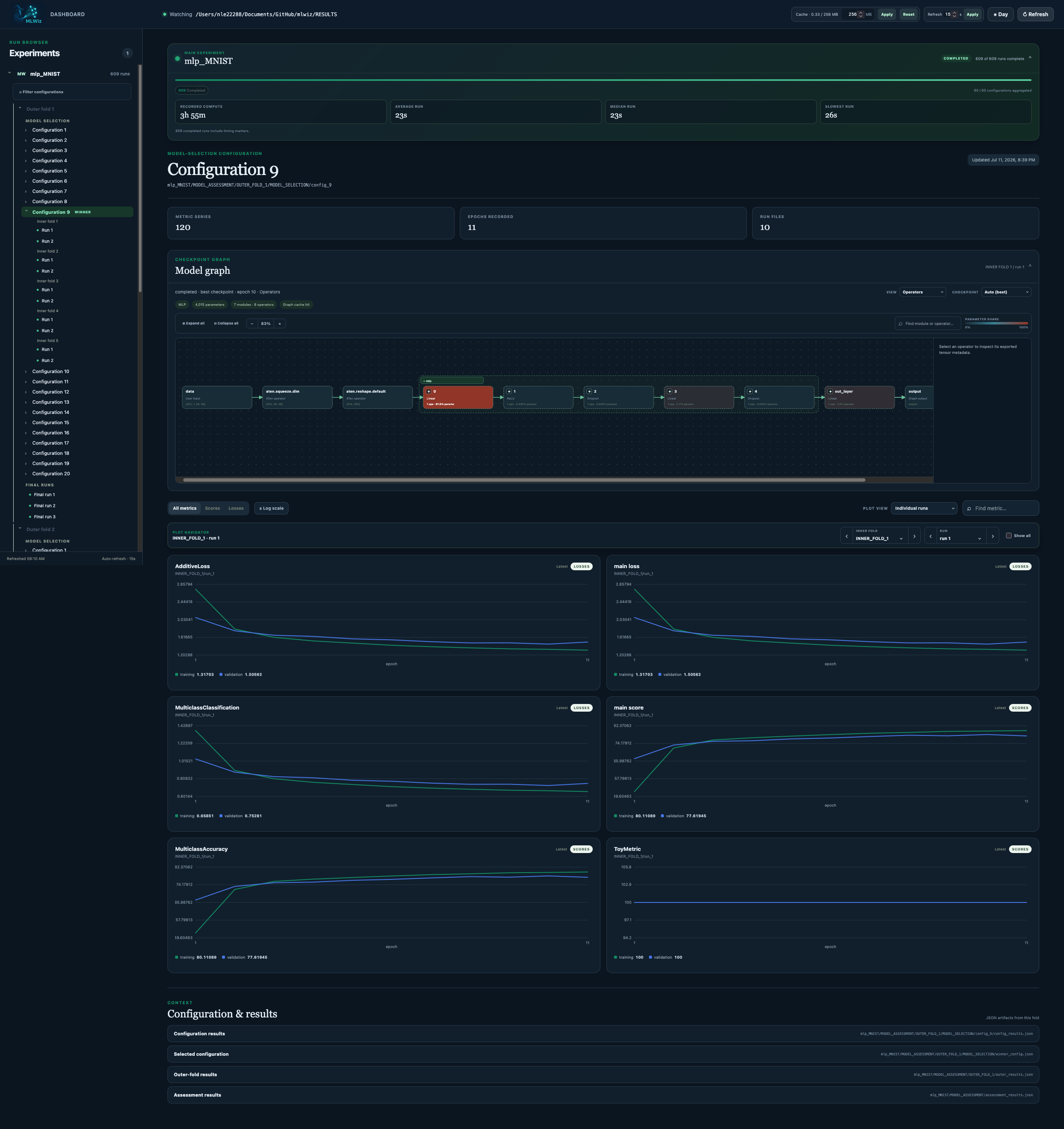
MLWiz includes a local, read-only visualization dashboard for exploring running
and completed experiments. It mirrors the model-selection and risk-assessment
hierarchy, plots score and loss histories, summarizes run progress and timing,
provides checkpoint-based model graph views, and includes a dedicated live
model-selection analysis workspace for comparing metrics across tried
hyperparameters. Every rendered chart has a </> Python action that generates
standalone Matplotlib + tueplots code with the displayed data. Start it with:
mlwiz-dashboard --logdir RESULTS
See the dashboard section for its filtering, comparison, caching, and model-inspection features.
To share a dashboard without sharing the project, click Export all in the
dashboard. The resulting .mlwiz file contains normalized metric histories,
metadata, filters, and navigation state for all experiments under --logdir;
it does not contain checkpoints, executable Python objects, or operator graphs.
A recipient with MLWiz installed can open it with:
mlwiz-dashboard-import shared-view.mlwiz --open
The same archive can be produced without a browser:
mlwiz-dashboard-export --logdir RESULTS --output shared-view.mlwiz
Optionally pass a dashboard-relative path to export only the experiment that contains that configuration or run:
mlwiz-dashboard-export --logdir RESULTS \
  --path mlp_MNIST/MODEL_ASSESSMENT/OUTER_FOLD_1/final_run1 \
  --output shared-view.mlwiz
See the peer-sharing guide for the complete sender and recipient workflow, archive contents, privacy considerations, and scoped exports.
🧭 Navigating the CLI (non-debug mode)
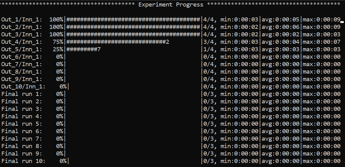
Example of the global view CLI:
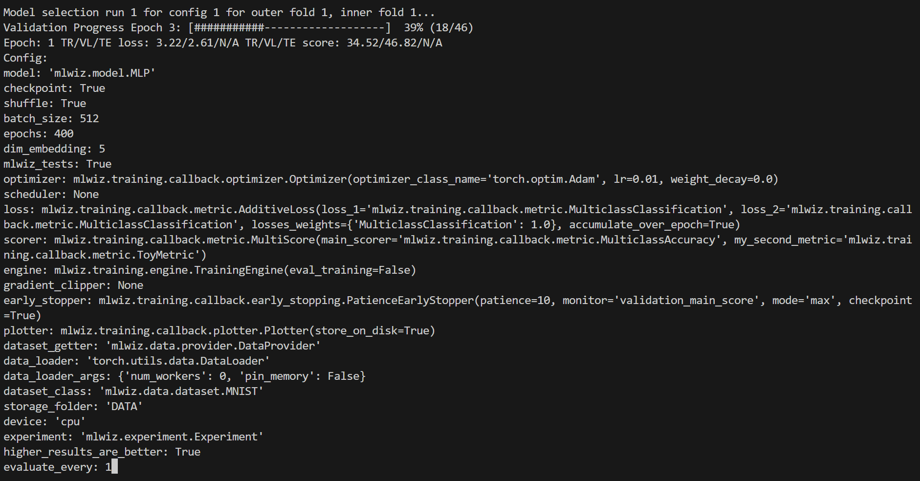
Specific views can be accessed, e.g. to visualize a specific model run:
:<outer_fold> <inner_fold> <config_id> <run_id>
…or, analogously, a risk assessment run:
:<outer_fold> <run_id>
Here is how it will look like
Handy commands:
:  # or :g or :global (back to global view)
:r # or :refresh (refresh the screen)
You can use left-right arrows to move across configurations, and up-down arrows to switch between model selection and risk assessment runs.
🧩 Architecture (High-Level)
MLWiz is built around two YAML files and a small set of composable components:
data.yml ──► mlwiz-data ──► processed dataset + .splits
exp.yml  ──► mlwiz-exp  ──► Ray workers
                      ├─ inner folds: model selection (best hyperparams)
                      └─ outer folds: risk assessment (final scores)
- 🧰 Data pipeline:
mlwiz-datainstantiates your dataset class and writes a.splitsfile for hold-out / (nested) CV. - 🧪 Search space:
grid:andrandom:sections expand into concrete hyperparameter configurations. - 🛰️ Orchestration: the evaluator schedules training runs with Ray across CPU/GPU (or a Ray cluster).
- 🏗️ Execution: each run builds a model + training engine from dotted paths, then logs artifacts and returns structured results.
⚙️ Configuration At A Glance
MLWiz expects:
- 🗂️ one YAML for data + splits
- 🧾 one YAML for experiment + search space
Minimal data config:
splitter:
  splits_folder: DATA_SPLITS/
  class_name: mlwiz.data.splitter.Splitter
  args:
    n_outer_folds: 3
    n_inner_folds: 2
    seed: 42

dataset:
  class_name: mlwiz.data.dataset.MNIST
  args:
    storage_folder: DATA/
Experiment configs use five required global sections plus exactly one model-selection section:
dataset:
  storage_folder: DATA
  dataset_class: mlwiz.data.dataset.MNIST
  data_splits_file: DATA_SPLITS/MNIST/MNIST_outer3_inner2.splits

resources:
  device: cpu
  max_cpus: 8
  max_gpus: 0
  gpus_per_task: 0

reproducibility:
  seed: 42

data_loading:
  dataset_getter: mlwiz.data.provider.DataProvider
  data_loader:
    class_name: torch.utils.data.DataLoader
    args:
      num_workers: 0
      pin_memory: false

experiment:
  result_folder: RESULTS
  exp_name: mlp
  experiment: mlwiz.experiment.Experiment
  model_selection_criteria:
    - metric: main_score
      direction: max
  evaluate_every: 1
  risk_assessment_training_runs: 3
  model_selection_training_runs: 2

grid:
  model: mlwiz.model.MLP
  epochs: 400
  batch_size: 512
  optimizer:
    class_name: mlwiz.training.callback.optimizer.Optimizer
    args:
      optimizer_class_name: torch.optim.Adam
      lr: 0.01
  loss: mlwiz.training.callback.metric.MulticlassClassification
  scorer: mlwiz.training.callback.metric.MulticlassAccuracy
  engine: mlwiz.training.engine.TrainingEngine
When mixed_precision: true is used on CPU, requesting
mixed_precision_dtype: torch.float16 is automatically converted to
torch.bfloat16.
higher_results_are_better remains available as a legacy shortcut for
main_score, but it cannot be set together with model_selection_criteria.
See examples/ for complete configs (including random/Bayesian search, schedulers, early stopping, and more).
Modular configuration groups
MLWiz composes YAML files using an ordered Hydra-style defaults list. Global
defaults belong at the root; model-selection defaults belong inside grid,
random, or bayes:
MODEL_CONFIGS/
├── config_MLP.yml
├── dataset/
│   └── mnist.yml
├── resources/
│   └── cpu.yml
└── optimizer/
    ├── adam.yml
    └── adagrad.yml
# config_MLP.yml
defaults:
  - dataset: mnist
  - resources: cpu
  - reproducibility: default
  - data_loading: torch
  - experiment: default
  - _self_

experiment:
  exp_name: mlp

grid:
  defaults:
    - optimizer:
        - adam
        - adagrad
    - search/mlp@_here_
    - _self_
  model: mlwiz.model.MLP
  epochs: 100
The terminology is precise:
- Defaults list: the ordered
defaults:sequence that tells MLWiz which files to compose. The directive itself is removed from the final config. - Config group: a directory of named alternatives.
dataset: mnistselectsdataset/mnist.ymland normally places its contents underdataset. _self_: the current file at that exact point in composition order. Values composed later override scalar/list values; dictionaries merge. If omitted,_self_is implicitly last.- Nested defaults: a
defaultslist insidegrid,random, orbayes. Its selected files are composed only into that search section, cleanly separating runtime settings from model selection. - Package override:
group@package: optionchanges where a selected file is placed. For example,optimizer@training.optimizer: adamtargetstraining.optimizerinstead ofoptimizer. _here_package: merges a selected mapping directly into the section containing the nested defaults.search/mlp@_here_contributesloss,scorer, andenginedirectly togrid._global_package: at the root defaults list, removes the normal group wrapper and merges a mapping into the root configuration. Use it for a file that already contains complete top-level sections.- Nested config defaults: a selected config file may define its own
defaults; MLWiz resolves those recursively and rejects cycles.
Selecting multiple files from a search config group concatenates every alternative. Grid search expands all of them; random and Bayesian search treat them as categorical alternatives and still resolve samplers nested inside the selected configuration.
Paths are relative to the file declaring defaults; a leading / resolves
from the main config directory. Flat experiment configurations are intentionally
rejected with an MLWiz 1.7.0 migration error—there is no legacy fallback. See
examples/MODEL_CONFIGS/config_MLP.yml.
🧩 Custom Code Via Dotted Paths
Point YAML entries to your own classes (in your project). mlwiz-data and mlwiz-exp add the current working directory to sys.path, so this works out of the box:
grid:
  model: my_project.models.MyModel

dataset:
  dataset_class: my_project.data.MyDataset
📦 Outputs
Runs are written under RESULTS/:
| Output | Location |
|---|---|
| Aggregated outer-fold results | RESULTS/<exp_name>_<dataset>/MODEL_ASSESSMENT/assessment_results.json |
| Per-fold summaries | RESULTS/<exp_name>_<dataset>/MODEL_ASSESSMENT/OUTER_FOLD_k/outer_results.json |
| Model selection (inner folds + winner config) | .../MODEL_SELECTION/... |
| Final retrains with selected hyperparams | .../final_run*/ |
When a Plotter callback is configured, each training run writes dashboard
histories to <run_dir>/metrics_data.torch.
MLWiz Dashboard
MLWiz includes a local, read-only experiment dashboard tailored to the result hierarchy above. Start it from the project that contains your results:
mlwiz-dashboard --logdir RESULTS
The dashboard adds the current directory to Python's import path so model
classes referenced by project-local dotted paths can be reconstructed. When
starting it elsewhere, pass the source directory explicitly with
--project-root /path/to/project.
Open the URL printed by the command (by default
http://127.0.0.1:6006). The run browser groups results by experiment, outer
fold, model-selection configuration, inner fold, and final run. Selecting a
configuration compares all of its child runs; selecting an individual run
shows only that run. Score and loss histories are refreshed after every epoch
by default. Set store_every_N_epochs to a larger value to reduce the write
frequency. To additionally record training-batch histories, configure
store_every_N_steps with a positive integer; the dashboard then exposes an
Epoch / Step history selector and plots the sampled global step numbers.
Hover over a chart to inspect the values at one epoch or sampled training step.
New sampled-step histories also record their wall-clock times, so the hover
readout shows the local date and time beside the step number. Aggregate trend
points show the recording-time range across their contributing runs. Older
metric artifacts without timestamps retain the step-only readout.
On any 2D trend chart, drag a rectangle over the plotting area to zoom into
that X/Y region. Box zoom can be repeated; Zoom out returns through the
selected regions one level at a time. The existing 3D controls continue to use
drag rotation and mouse-wheel zoom.
Use Smoothing to apply the same bias-corrected exponential moving average
used by TensorBoard; 0 leaves the curve unchanged, while higher values reduce
short-term noise and retain a faint raw trace for context. The mirrored control
in Model Selection Analysis applies the same value to 2D, 3D, and combined
trend curves and stays pinned above the analysis plots while you scroll. The
chosen value is preserved for the dashboard session and included with
reproducible plot exports.
Use Remove outliers in a mean ± standard-deviation Run Explorer view, or on
an individual Model Selection Analysis plot, to exclude values outside Tukey's
1.5×IQR fences. Trend filtering is performed independently at each epoch or
sampled step within each plotted group; distributions are filtered within each
hyperparameter bucket. At least four finite samples are required, removed-value
counts are shown in the plot, and individual run histories and stored artifacts
remain unchanged. Reproducible plot exports contain the displayed, filtered data.
The Log scale control uses a conventional base-10 logarithmic axis when
every displayed value is positive. If zero or negative values are present, it
automatically uses an adaptive symmetric-log axis: a small neighborhood around
zero stays linear and larger magnitudes are logarithmic. The linear threshold
is derived from the displayed data and limited to six decades below its largest
magnitude, so the behavior is independent of whether a metric is naturally
measured near 1, 0.01, or another scale. Each experiment has its own lazy-loaded
configuration filter: choose any discovered score or loss and compare its
training or validation value with a threshold using ≥ or ≤, or choose a
hyper-parameter and match one of its tried values using = or ≠. Nested
hyper-parameters are displayed as dotted paths such as optimizer.lr; parameters
with only one discovered value are omitted. Multiple metric and hyper-parameter
conditions can be combined with AND or OR. Completed
experiments use their aggregated metric results; running experiments use the
latest values available in metrics_data.torch and configuration values from
live run manifests when necessary. Remove the final condition with ×, or
use Clear, to return to the unfiltered view while keeping the filter controls
open. While a filter is active, final runs are
hidden, Model Selection Analysis plots and exports include only matching
configurations, and an experiment with no matching configuration shows only its
filter controls.
Model Selection Analysis
The separate Model Selection Analysis tab compares configurations and runs inside one selected outer-fold/inner-fold pair. It offers only hyperparameters for which more than one value was actually tried. Add any number of plots to the workspace: each plot retains its own grouping, dimensionality, output, display, expansion, and camera controls, and can be removed directly from its card. For a 2D Trend or Metric-vs-Hyperparameter plot, choose None — average all runs under Group by to collapse every run into one aggregate. Combined Trends and 3D plots require real grouping parameters and do not offer None.
- Trend Plots show epoch- or sampled-step-wise mean ± standard deviation for runs sharing a hyperparameter value. Select the unit for the next plot or change it independently on an existing card. Add a second hyperparameter for a 3D view, or enable the persistent per-card Log scale control. It uses a conventional logarithmic axis for all-positive values and automatically falls back to the adaptive symmetric-log axis when zero or negative values occur. In 2D, Group by None produces one mean curve and deviation band across every run.
- Combined Trends place epoch or sampled step and two recorded quantities on a 3D trajectory grouped by one hyperparameter. Their Log scale control selects the appropriate logarithmic mode independently for each recorded-quantity axis.
- Metric vs Hyper-Parameter compares each run's best-checkpoint metric value, falling back to its last recorded value. It supports 2D histograms, 3D heatmap bars for two hyperparameters, violin distributions with optional raw points, automatic logarithmic/symmetric-log scaling, Markdown tables, and a 2D all-runs aggregate.
Numeric custom histories in metrics_data.torch are discovered alongside
losses and scores. Rectangular epoch-by-layer/component data is treated as one
family: selecting it overlays every related layer or component in one plot with
a legend by default. Use the per-card Series: Together / Separate control to
switch between that shared view and one plot per family member. The same control
is available for combined trends that resolve to multiple quantity pairs. Long
chart legends are capped and scroll vertically; hover over or keyboard-focus a
legend entry to emphasize its line and fade the others. All 3D views support
drag rotation, mouse-wheel zoom, X/Y/Z alignment, hover values, and per-card
expand/shrink controls. See the
model-selection analysis tutorial
for the aggregation rules, plot semantics, and custom WidthPlotter example.
Exporting reproducible plot code
Every rendered metric or model-selection chart includes a </> Python button.
Click it to open a live preview of a standalone script containing the normalized
data currently displayed by that chart. The generated code uses Matplotlib and
tueplots to reproduce line and
uncertainty-band charts, histograms, violin plots, heatmap bars, and 3D views.
The export dialog lets you choose a conference or journal bundle, single-column
or full-width sizing, PDF/PNG/SVG/PGF output, grid/title/legend visibility, and
LaTeX or standard Matplotlib text rendering. Paul Tol muted is the default
colorblind-safe palette; other colorblind-safe and tueplots palettes are
available. These choices persist across browser sessions. Use Copy code or
Download .py, then install the script dependencies if needed:
uv add matplotlib numpy tueplots
LaTeX rendering is disabled by default and requires a working local TeX
installation when enabled. The script saves the figure in the selected format
and also opens it with plt.show().
The header also provides a persistent refresh-interval setting and a day/dark theme toggle, plus persistent font-family and font-size controls. Dark mode is the default.
Above the selected configuration or run, a collapsible overview summarizes its
parent experiment only: completed, running, queued, and failed runs; aggregated
configurations; recorded compute time; average and median run duration; and an
estimated remaining compute budget. Timing comes from the profiler markers in
each experiment.log. The remaining estimate is deliberately reported as
compute time because parallel execution may complete in less wall-clock time.
The metadata section also exposes the resolved configuration associated with a
selected run or configuration as a dedicated, collapsible JSON inspector. Run
configurations come from model_manifest.json; completed configuration entries
come from config_results.json, with a live-run manifest fallback while an
experiment is still running. Nested fields in these dedicated configuration
inspectors are expanded automatically on first view; manually collapsed fields
retain their state across refreshes.
The collapsible Model graph panel loads graph information only when opened.
For a running job it reads last_checkpoint.pth; for a completed job it prefers
best_checkpoint.pth, falling back to the other checkpoint when necessary. A
checkpoint selector can explicitly display Best or Last whenever that file
exists, while Auto retains the status-based policy. When metric plots are
grouped by inner fold, the panel has its own Run selector so any run in the
focused fold can be inspected independently of the plots.
The View selector offers two representations. Architecture reconstructs the
CPU module hierarchy from model_manifest.json, with a checkpoint-parameter
hierarchy fallback for older runs. Operators uses torch.export to trace the
selected checkpoint and displays the resulting dataflow as individual ATen
operations, including output shapes and originating module paths when export
provides them. The initial view collapses those operations into top-level module
nodes connected by directional arrows, making the actual forward-pass DAG
visible. Expand a module to reveal its child modules, then expand again to reach
the ATen operations inside it; expanded module boundaries remain on the canvas
and can be collapsed in place. Use the −, percentage, and + controls (or
the mouse wheel anywhere inside the graph) to zoom around the pointer. Drag the
empty canvas to pan horizontally or vertically, and drag any module/operator box
to place it manually; custom zoom, expansion, and box positions persist for that
run and checkpoint view.
New runs record only data-free metadata for the first forward input in
model_graph_input_spec.json; no training values are stored. Tensor inputs use
their shape and dtype. PyG/custom input models can implement
model_graph_input_spec, supports_model_graph_input, and
model_graph_export_adapter to provide synthetic tensor inputs for Operators.
Adapters may select proxy tracing for scientific models whose TorchScript-class
metadata can not be flattened by torch.export.
Enable checkpoint: true to produce last checkpoints; best checkpoints are
available when the configured early stopper stores them.
Model weights and run metadata use the stable last_checkpoint.pth and
best_checkpoint.pth names. Resumable optimizer, scheduler, and AMP scaler
state is stored separately in last_optimizer_checkpoint.pth and
best_optimizer_checkpoint.pth; the dashboard reads only the model files.
Pre-1.7 bundled checkpoints remain resumable when no optimizer file is present.
To bound temporary memory pressure, the graph is not loaded when the checkpoint
file itself is larger than the cache ceiling configured in the dashboard.
Oversized Best/Last choices remain visible but disabled in the selector.
The graph explorer groups modules into a collapsible hierarchy, supports
expand/collapse-all, search, and a flattened leaf-module view. Block color
represents the parameters contained by that block and its descendants relative
to the model's total parameter count; the inspector shows the exact count and
percentage for the selected block. Operator parameter placeholders use the same
relative parameter coloring, while ordinary operations remain at the zero-share
end of the scale.
The charts read metrics_data.torch. Configure the Plotter callback to write
this artifact (metric storage is enabled by default):
plotter: mlwiz.training.callback.plotter.Plotter
Step histories are opt-in. This example records and flushes one training-batch sample every 10 optimizer steps while retaining the default epoch histories:
plotter:
  class_name: mlwiz.training.callback.plotter.Plotter
  args:
    store_every_N_steps: 10
Leave store_every_N_steps unset (or set it to null) to store epoch metrics
only. store_every_N_epochs continues to control epoch-based disk flushes.
With step histories enabled, Plotter persists each sample's Unix timestamp
and also the exact global step at each completed epoch. Resuming an epoch
checkpoint discards any later samples and timestamps from an interrupted
partial epoch, then records their replacement values at the same global step
numbers.
Use mlwiz-dashboard --help for host, port, and browser-opening options.
Portable dashboards can be shared without copying the result directory or
custom model code. Use Export all in the dashboard or
mlwiz-dashboard-export --logdir RESULTS --output shared.mlwiz, then have the
recipient run mlwiz-dashboard-import shared.mlwiz --open. See the
peer-sharing guide for details and privacy considerations.
Metric artifacts are loaded only when a configuration or run is selected. The
dashboard keeps normalized histories in a least-recently-used cache (256 MB by
default); its memory limit can be changed from the dashboard header, and 0
disables caching. The limit applies only to retained cache entries: a selected
configuration is still loaded and displayed even when it is larger than the
configured buffer. Lazily generated model graphs share this bounded cache and
are also cleared by the header's cache-reset button.
🛠️ Utilities
🗂️ Config Management (CLI)
Duplicate a base experiment config across multiple datasets:
mlwiz-config-duplicator --base-exp-config base.yml --data-config-files data1.yml data2.yml
📊 Post-process Results (Python)
Filter configurations from a MODEL_SELECTION/ folder and convert them to a DataFrame:
from mlwiz.evaluation.util import retrieve_experiments, filter_experiments, create_dataframe

configs = retrieve_experiments(
    "RESULTS/mlp_MNIST/MODEL_ASSESSMENT/OUTER_FOLD_1/MODEL_SELECTION/"
)
filtered = filter_experiments(configs, logic="OR", parameters={"lr": 0.001})
df = create_dataframe(
    config_list=filtered,
    key_mappings=[("lr", float), ("avg_validation_score", float)],
)
Export aggregated assessment results to LaTeX:
from mlwiz.evaluation.util import create_latex_table_from_assessment_results

experiments = [
    ("RESULTS/mlp_MNIST", "MLP", "MNIST"),
    ("RESULTS/dgn_PROTEINS", "DGN", "PROTEINS"),
]

latex_table = create_latex_table_from_assessment_results(
    experiments,
    metric_key="main_score",
    no_decimals=3,
    model_as_row=True,
    use_single_outer_fold=False,
)
print(latex_table)
Compare statistical significance between models (Welch t-test):
from mlwiz.evaluation.util import statistical_significance

reference = ("RESULTS/mlp_MNIST", "MLP", "MNIST")
competitors = [
    ("RESULTS/baseline1_MNIST", "B1", "MNIST"),
    ("RESULTS/baseline2_MNIST", "B2", "MNIST"),
]

df = statistical_significance(
    highlighted_exp_metadata=reference,
    other_exp_metadata=competitors,
    metric_key="main_score",
    set_key="test",
    confidence_level=0.95,
)
print(df)
🔍 Load a Trained Model (Notebook-friendly)
Load the best configuration for a fold, instantiate dataset/model, and restore a checkpoint:
from mlwiz.evaluation.util import (
    retrieve_best_configuration,
    instantiate_dataset_from_config,
    instantiate_model_from_config,
    load_checkpoint,
)

config = retrieve_best_configuration(
    "RESULTS/mlp_MNIST/MODEL_ASSESSMENT/OUTER_FOLD_1/MODEL_SELECTION/"
)
dataset = instantiate_dataset_from_config(config)
model = instantiate_model_from_config(config, dataset)
load_checkpoint(
    "RESULTS/mlp_MNIST/MODEL_ASSESSMENT/OUTER_FOLD_1/final_run1/best_checkpoint.pth",
    model,
    device="cpu",
)
For more post-processing helpers, see the tutorial: https://mlwiz.readthedocs.io/en/stable/tutorial.html
🤝 Contributing
See CONTRIBUTING.md.
📄 License
BSD-3-Clause. See LICENSE.
Release history Release notifications | RSS feed


Download files
Download the file for your platform. If you're not sure which to choose, learn more about installing packages.
Source Distribution
Built Distribution
Filter files by name, interpreter, ABI, and platform.
If you're not sure about the file name format, learn more about wheel file names.
Copy a direct link to the current filters
File details
Details for the file mlwiz-1.7.4.tar.gz.
File metadata
- Download URL: mlwiz-1.7.4.tar.gz
- Upload date:
- Size: 2.4 MB
- Tags: Source
- Uploaded using Trusted Publishing? No
- Uploaded via: twine/6.1.0 CPython/3.13.13
File hashes
| Algorithm | Hash digest | |
|---|---|---|
| SHA256 |
dcb2d05819cd6378eebdc4b5ff62c13dd46b62cd157cd28abefdb0338cfc347c
|
|
| MD5 |
878011e158bde7bff35485d5dc1d8a32
|
|
| BLAKE2b-256 |
9bd96e106ba6866e1c25080415f0a1f4b10631664b1e03ede8860673ece93639
|
File details
Details for the file mlwiz-1.7.4-py3-none-any.whl.
File metadata
- Download URL: mlwiz-1.7.4-py3-none-any.whl
- Upload date:
- Size: 2.4 MB
- Tags: Python 3
- Uploaded using Trusted Publishing? No
- Uploaded via: twine/6.1.0 CPython/3.13.13
File hashes
| Algorithm | Hash digest | |
|---|---|---|
| SHA256 |
9bc916fc927f0ad24aa4600855c46ebee1d4bdd2cd8587288c309f6dd9ad6957
|
|
| MD5 |
65d7aba08a744f8a31ee1f7eb967d88a
|
|
| BLAKE2b-256 |
9117a24d407ea332d9ced533ef8ce51885440ff787a9b25022b5d831d6c7b825
|






