Modern difference-in-differences estimators.
Verified details
These details have been verified by PyPIProject links
GitHub Statistics
Maintainers

Project description


ModernDiD is a scalable, GPU-accelerated difference-in-differences library for Python. It consolidates modern DiD estimators from leading econometric research and various R and Stata packages into a single framework with a consistent API. Runs on a single machine, NVIDIA GPUs, and distributed Spark and Dask clusters.
Features
- DiD Estimators - Staggered DiD, Doubly Robust DiD, Continuous DiD, Triple DiD, Intertemporal DiD, Honest DiD.
- Dataframe agnostic - Pass any Arrow-compatible DataFrame such as polars, pandas, pyarrow, duckdb, and more powered by narwhals.
- Distributed computing - Scale to billions of observations across Spark and Dask clusters. Pass a distributed DataFrame and the backend activates transparently.
- Fast computation - Polars for internal data wrangling, NumPy vectorization, Numba JIT compilation, and threaded parallel compute.
- GPU acceleration - Optional CuPy-accelerated estimation on NVIDIA GPUs, with multi-GPU scaling in distributed environments.
- Native plots - Built-in visualizations powered by plotnine, returning standard
ggplotobjects you can customize with the full grammar of graphics. - Robust inference - Analytical standard errors, bootstrap (weighted and multiplier), and simultaneous confidence bands.
For detailed documentation, including user guides and API reference, see moderndid.readthedocs.io.
Installation
uv pip install moderndid        # Core estimators (did, drdid, didinter, didtriple)
uv pip install moderndid[all]   # All estimators, plots, numba, spark, dask (excludes gpu)
Some estimators and features require additional dependencies that are not installed by default. Extras are additive and build on the base install, so you always get the core estimators (att_gt, drdid, did_multiplegt, ddd) plus whatever extras you specify:
didcont- Continuous treatment DiD (cont_did)didhonest- Sensitivity analysis (honest_did)plots- Batteries-included plotsnumba- Faster bootstrap inferencespark- Distributed estimation via PySparkdask- Distributed estimation via Daskgpu- GPU-accelerated estimation (requires CUDA)
uv pip install moderndid[didcont,plots]   # Combine multiple extras
uv pip install moderndid[gpu,spark]       # GPU + distributed
Quick Start
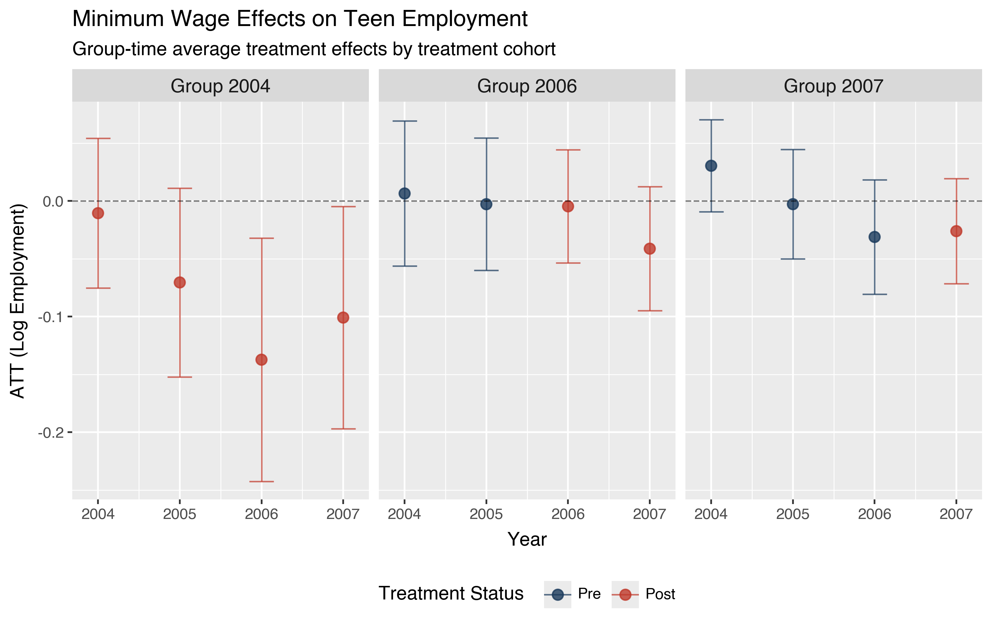
This example uses county-level teen employment data to estimate the effect of minimum wage increases. States adopted higher minimum wages at different times (2004, 2006, or 2007), making this a staggered adoption design.
The att_gt() function estimates the average treatment effect for each group g (defined by when units were first treated) at each time period t. We use the doubly robust estimator, which combines outcome regression and propensity score weighting to provide consistent estimates if either model is correctly specified.
import moderndid as did

data = did.load_mpdta()

attgt_result = did.att_gt(
    data=data,
    yname="lemp",
    tname="year",
    idname="countyreal",
    gname="first.treat",
    est_method="dr",
)
print(attgt_result)
==============================================================================
 Group-Time Average Treatment Effects
==============================================================================

┌───────┬──────┬──────────┬────────────┬────────────────────────────┐
│ Group │ Time │ ATT(g,t) │ Std. Error │ [95% Pointwise Conf. Band] │
├───────┼──────┼──────────┼────────────┼────────────────────────────┤
│  2004 │ 2004 │  -0.0105 │     0.0233 │ [-0.0561,  0.0351]         │
│  2004 │ 2005 │  -0.0704 │     0.0310 │ [-0.1312, -0.0097] *       │
│  2004 │ 2006 │  -0.1373 │     0.0364 │ [-0.2087, -0.0658] *       │
│  2004 │ 2007 │  -0.1008 │     0.0344 │ [-0.1682, -0.0335] *       │
│  2006 │ 2004 │   0.0065 │     0.0233 │ [-0.0392,  0.0522]         │
│  2006 │ 2005 │  -0.0028 │     0.0196 │ [-0.0411,  0.0356]         │
│  2006 │ 2006 │  -0.0046 │     0.0178 │ [-0.0394,  0.0302]         │
│  2006 │ 2007 │  -0.0412 │     0.0202 │ [-0.0809, -0.0016] *       │
│  2007 │ 2004 │   0.0305 │     0.0150 │ [ 0.0010,  0.0600] *       │
│  2007 │ 2005 │  -0.0027 │     0.0164 │ [-0.0349,  0.0294]         │
│  2007 │ 2006 │  -0.0311 │     0.0179 │ [-0.0661,  0.0040]         │
│  2007 │ 2007 │  -0.0261 │     0.0167 │ [-0.0587,  0.0066]         │
└───────┴──────┴──────────┴────────────┴────────────────────────────┘

------------------------------------------------------------------------------
 Signif. codes: '*' confidence band does not cover 0

 P-value for pre-test of parallel trends assumption:  0.1681

------------------------------------------------------------------------------
 Data Info
------------------------------------------------------------------------------
 Control Group:  Never Treated
 Anticipation Periods:  0

------------------------------------------------------------------------------
 Estimation Details
------------------------------------------------------------------------------
 Estimation Method:  Doubly Robust

------------------------------------------------------------------------------
 Inference
------------------------------------------------------------------------------
 Significance level: 0.05
 Analytical standard errors
==============================================================================
 Reference: Callaway and Sant'Anna (2021)
ModernDiD provides "batteries-included" plotting functions (plot_event_study, plot_gt, plot_agg, and more) as well as data converters for building custom figures with plotnine. Since all plot functions return ggplot objects, you can restyle them with the full grammar of graphics:
from plotnine import element_text, labs, theme, theme_gray

p = did.plot_gt(attgt_result, ncol=3)
p = (p
    + labs(
        x="Year",
        y="ATT (Log Employment)",
        title="Minimum Wage Effects on Teen Employment",
        subtitle="Group-time average treatment effects by treatment cohort",
    )
    + theme_gray()
    + theme(
        legend_position="bottom",
        strip_text=element_text(size=11, weight="bold"),
    )
)
While group-time effects are useful, they can be difficult to summarize when there are many groups and time periods. The aggte function aggregates these into more interpretable summaries. Setting type="dynamic" produces an event study that shows how effects evolve relative to treatment timing:
event_study = did.aggte(attgt_result, type="dynamic")
print(event_study)
==============================================================================
 Aggregate Treatment Effects (Event Study)
==============================================================================

 Overall summary of ATT's based on event-study/dynamic aggregation:

┌─────────┬────────────┬────────────────────────┐
│     ATT │ Std. Error │ [95% Conf. Interval]   │
├─────────┼────────────┼────────────────────────┤
│ -0.0772 │     0.0200 │ [ -0.1164,  -0.0381] * │
└─────────┴────────────┴────────────────────────┘


 Dynamic Effects:

┌────────────┬──────────┬────────────┬────────────────────────────┐
│ Event time │ Estimate │ Std. Error │ [95% Pointwise Conf. Band] │
├────────────┼──────────┼────────────┼────────────────────────────┤
│         -3 │   0.0305 │     0.0150 │ [-0.0078,  0.0688]         │
│         -2 │  -0.0006 │     0.0133 │ [-0.0344,  0.0333]         │
│         -1 │  -0.0245 │     0.0142 │ [-0.0607,  0.0118]         │
│          0 │  -0.0199 │     0.0118 │ [-0.0501,  0.0102]         │
│          1 │  -0.0510 │     0.0169 │ [-0.0940, -0.0079] *       │
│          2 │  -0.1373 │     0.0364 │ [-0.2301, -0.0444] *       │
│          3 │  -0.1008 │     0.0344 │ [-0.1883, -0.0133] *       │
└────────────┴──────────┴────────────┴────────────────────────────┘

------------------------------------------------------------------------------
 Signif. codes: '*' confidence band does not cover 0

------------------------------------------------------------------------------
 Data Info
------------------------------------------------------------------------------
 Control Group: Never Treated
 Anticipation Periods: 0

------------------------------------------------------------------------------
 Estimation Details
------------------------------------------------------------------------------
 Estimation Method: Doubly Robust

------------------------------------------------------------------------------
 Inference
------------------------------------------------------------------------------
 Significance level: 0.05
 Analytical standard errors
==============================================================================
 Reference: Callaway and Sant'Anna (2021)
Event time 0 is the on-impact effect, negative event times are pre-treatment periods, and positive event times are post-treatment periods. Pre-treatment effects near zero support the parallel trends assumption, while post-treatment effects show how the impact evolves over time.
Data converters make it easy to overlay estimates from different estimators. The figure below compares the Callaway and Sant'Anna estimates against a standard TWFE event study estimated with pyfixest. See the Plotting Guide for the full code and more examples.
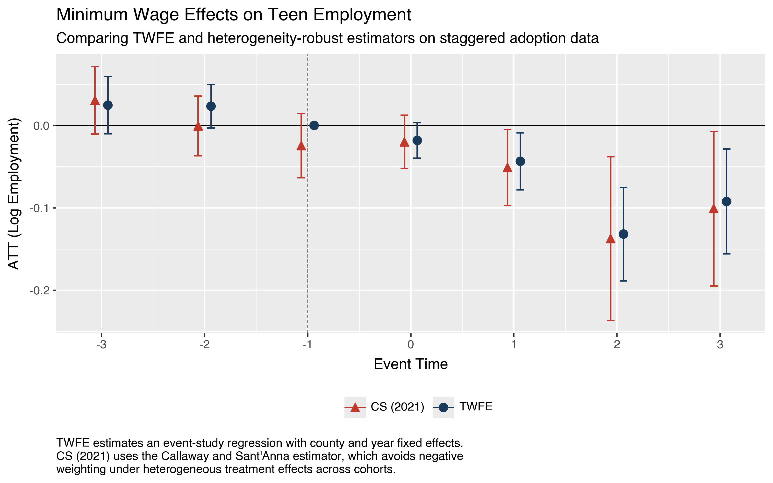
Consistent API
All estimators share a unified interface. Pass any Arrow PyCapsule-compatible DataFrame (polars, pandas, pyarrow, duckdb, and others) and estimation works the same way:
result = did.att_gt(data, yname="y", tname="t", idname="id", gname="g", ...)
result = did.ddd(data, yname="y", tname="t", idname="id", gname="g", pname="p", ...)
result = did.cont_did(data, yname="y", tname="t", idname="id", gname="g", dname="dose", ...)
result = did.drdid(data, yname="y", tname="t", idname="id", treatname="treat", ...)
result = did.did_multiplegt(data, yname="y", tname="t", idname="id", dname="treat", ...)
Scaling Up
Distributed. Pass a Spark or Dask DataFrame and the distributed backend activates automatically. See the Distributed guide.
GPU. Pass backend="cupy" to offload estimation to NVIDIA GPUs. See the GPU guide and benchmarks.
from pyspark.sql import SparkSession
spark = SparkSession.builder.master("local[*]").getOrCreate()
result = did.att_gt(data=spark.read.parquet("panel.parquet"),
                    yname="y", tname="t", idname="id", gname="g")
result = did.att_gt(data, yname="lemp", tname="year", idname="countyreal",
                    gname="first.treat", backend="cupy")
Example Datasets
did.load_mpdta()       # County teen employment
did.load_nsw()         # NSW job training program
did.load_ehec()        # Medicaid expansion
did.load_engel()       # Household expenditure
did.load_favara_imbs() # Bank lending
did.load_cai2016()     # Crop insurance
Synthetic data generators are also available for simulations and benchmarking:
did.gen_did_scalable()           # Staggered DiD panel
did.simulate_cont_did_data()     # Continuous treatment DiD
did.gen_dgp_2periods()           # Two-period triple DiD
did.gen_dgp_mult_periods()       # Staggered triple DiD
did.gen_dgp_scalable()           # Large-scale triple DiD
Planned Development
moderndid.didml— Machine learning approaches to DiD (Hatamyar et al., 2023)moderndid.drdidweak— Robust to weak overlap (Ma et al., 2023)moderndid.didcomp— Compositional changes in repeated cross-sections (Sant'Anna & Xu, 2025)moderndid.didimpute— Imputation-based estimators (Borusyak, Jaravel, & Spiess, 2024)moderndid.didbacon— Goodman-Bacon decomposition (Goodman-Bacon, 2019)moderndid.didlocal— Local projections DiD (Dube et al., 2025)moderndid.did2s— Two-stage DiD (Gardner, 2021)moderndid.etwfe— Extended two-way fixed effects (Wooldridge, 2021; Wooldridge, 2023)moderndid.functional— Specification tests (Roth & Sant'Anna, 2023)
Acknowledgements
ModernDiD would not be possible without the researchers who developed the underlying econometric methods and implemented them in various R and Stata packages. See our Acknowledgements page for a full list of the software, packages, and papers that have influenced this project.
Citation
If you use ModernDiD in your research, please cite it as:
@software{moderndid,
  author  = {{The ModernDiD Authors}},
  title   = {{ModernDiD: Scalable, GPU-Accelerated Difference-in-Differences for Python}},
  year    = {2025},
  url     = {https://github.com/jordandeklerk/moderndid}
}
Project details
Verified details
These details have been verified by PyPIProject links
GitHub Statistics
Maintainers


Download files
Download the file for your platform. If you're not sure which to choose, learn more about installing packages.
Source Distribution
Built Distribution
Filter files by name, interpreter, ABI, and platform.
If you're not sure about the file name format, learn more about wheel file names.
Copy a direct link to the current filters
File details
Details for the file moderndid-0.1.1.tar.gz.
File metadata
- Download URL: moderndid-0.1.1.tar.gz
- Upload date:
- Size: 1.4 MB
- Tags: Source
- Uploaded using Trusted Publishing? Yes
- Uploaded via: twine/6.1.0 CPython/3.13.7
File hashes
| Algorithm | Hash digest | |
|---|---|---|
| SHA256 |
b84d02079fb121a0229693ba24504e45a1d5cb5a757837c77fd950dbdcbd7413
|
|
| MD5 |
7010a960b4505b71a6c694b819682fe5
|
|
| BLAKE2b-256 |
0acae0fcf139d2a5071b35c0379d1476a8ecfeba6bce06db73ddcfac45c7ad8a
|
Provenance
The following attestation bundles were made for moderndid-0.1.1.tar.gz:
Publisher:
publish.yml on jordandeklerk/moderndid
-
Statement:
-
Statement type:
https://in-toto.io/Statement/v1 -
Predicate type:
https://docs.pypi.org/attestations/publish/v1 -
Subject name:
moderndid-0.1.1.tar.gz -
Subject digest:
b84d02079fb121a0229693ba24504e45a1d5cb5a757837c77fd950dbdcbd7413 - Sigstore transparency entry: 999210612
- Sigstore integration time:
-
Permalink:
jordandeklerk/moderndid@edc5a4868864c4419389a3594683909ea070785c -
Branch / Tag:
refs/tags/v0.1.1 - Owner: https://github.com/jordandeklerk
-
Access:
public
-
Token Issuer:
https://token.actions.githubusercontent.com -
Runner Environment:
github-hosted -
Publication workflow:
publish.yml@edc5a4868864c4419389a3594683909ea070785c -
Trigger Event:
push
-
Statement type:
File details
Details for the file moderndid-0.1.1-py3-none-any.whl.
File metadata
- Download URL: moderndid-0.1.1-py3-none-any.whl
- Upload date:
- Size: 1.5 MB
- Tags: Python 3
- Uploaded using Trusted Publishing? Yes
- Uploaded via: twine/6.1.0 CPython/3.13.7
File hashes
| Algorithm | Hash digest | |
|---|---|---|
| SHA256 |
26377b624d7535f6b53b72afa889992af75123664df6bad30ba3e12a43f5d4e4
|
|
| MD5 |
0f3ff7d284115765c7a6ee251bfdc681
|
|
| BLAKE2b-256 |
3e3eaae5d6521426d2dcf912bba375cd472b48fbd80543393b7eb36e3deab133
|
Provenance
The following attestation bundles were made for moderndid-0.1.1-py3-none-any.whl:
Publisher:
publish.yml on jordandeklerk/moderndid
-
Statement:
-
Statement type:
https://in-toto.io/Statement/v1 -
Predicate type:
https://docs.pypi.org/attestations/publish/v1 -
Subject name:
moderndid-0.1.1-py3-none-any.whl -
Subject digest:
26377b624d7535f6b53b72afa889992af75123664df6bad30ba3e12a43f5d4e4 - Sigstore transparency entry: 999210691
- Sigstore integration time:
-
Permalink:
jordandeklerk/moderndid@edc5a4868864c4419389a3594683909ea070785c -
Branch / Tag:
refs/tags/v0.1.1 - Owner: https://github.com/jordandeklerk
-
Access:
public
-
Token Issuer:
https://token.actions.githubusercontent.com -
Runner Environment:
github-hosted -
Publication workflow:
publish.yml@edc5a4868864c4419389a3594683909ea070785c -
Trigger Event:
push
-
Statement type:


