Lightweight molecular coordinate workflows for descriptors, graph ML, and coarse-grained beads.
Verified details
These details have been verified by PyPIProject links
GitHub Statistics
Maintainers

Project description
MolScope


Lightweight molecular structure analysis, graph export, and coarse-graining in Python. MolScope is built around three polished workflows: turn coordinate files into descriptor tables, graph-ML inputs, or coarse-grained bead representations without pulling in a full simulation stack.
Read .xyz, .pdb, .cif and .sdf files, select and analyse atoms, and
visualise structures in 3D. Optional extras add Gemmi validation, RDKit chemical
features, PyTorch Geometric, DGL, and other backend integrations only when a
workflow needs them.
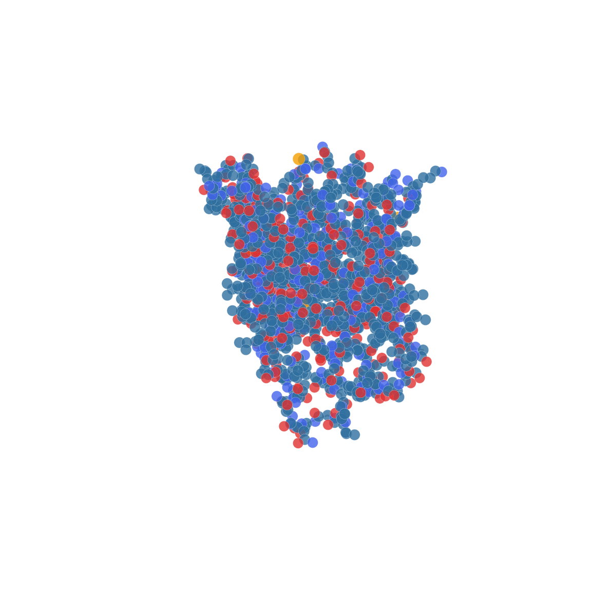
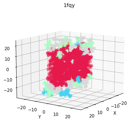
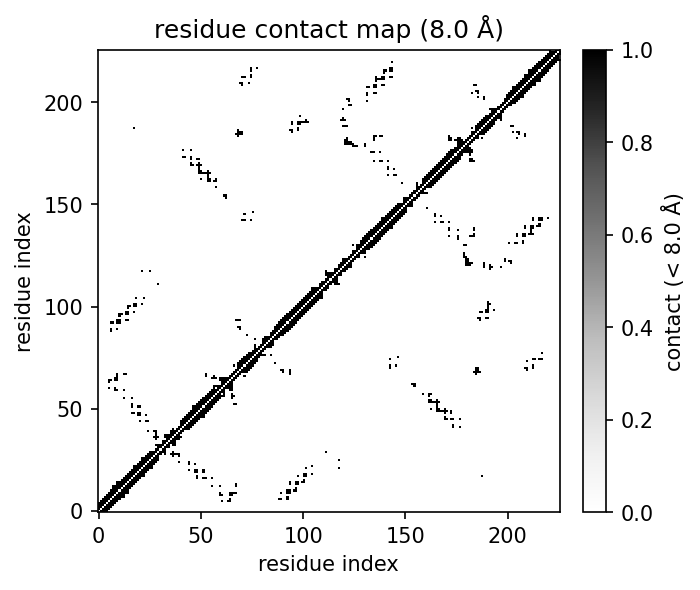
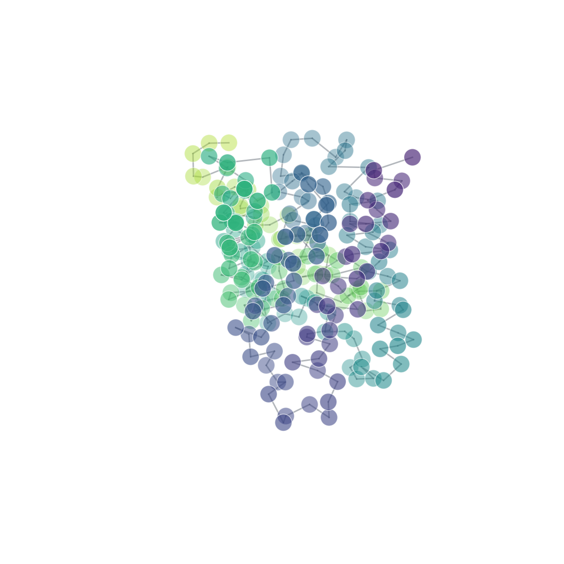
| 3D structure (element) | Secondary structure (DSSP) | Residue contact map | Coarse-grained beads |
|---|---|---|---|
 |
 |
 |
 |
Core workflows
| Workflow | Start here | Output |
|---|---|---|
| PDB to descriptors | docs/tutorials/pdb-to-descriptors.md |
Fixed-width structural and optional RDKit-backed feature tables for screening, QC, and classical ML. |
| PDB to graph/GNN | docs/tutorials/pdb-to-graph-gnn.md |
Atom/bond, residue-contact, and PyTorch Geometric-ready graph data for message-passing experiments. |
| PDB to coarse-grained beads | docs/tutorials/pdb-to-coarse-grained-beads.md |
Residue, simplified Martini-style, custom, and virtual-site bead models for inspection and graph prototyping. |
Who is this for?
- Students learning molecular-coordinate formats, structure analysis, and basic visualisation from readable Python code.
- Molecular modellers who want quick static-structure checks, selections, contact maps, and lightweight coarse-grained mapping prototypes.
- ML-for-molecules learners who need deterministic descriptors and graph exports before moving to larger chemistry or simulation frameworks.
Supporting capabilities
MolScope keeps the broad feature surface organized around those workflows:
- Input layer: read and write XYZ, PDB, mmCIF and SDF, preserve explicit bonds and charges where present, fetch structures from RCSB, and validate mmCIF files with optional Gemmi support.
- Structure analysis: select atoms by metadata, compute geometry, RMSD, contacts, contact maps, interfaces, binding sites, and ensemble summaries.
- Annotations and descriptors: run dependency-free secondary-structure assignment, native structural descriptors, and optional RDKit-backed chemistry descriptors.
- Representation outputs: export descriptor tables, atom/bond graphs, residue-contact graphs, and coarse-grained bead graphs to common ML backends.
- Inspection and automation: visualize with Matplotlib or py3Dmol and use the CLI for view, analyze, and export workflows.
Architecture
graph LR
    A[XYZ, PDB, mmCIF, SDF files] --> B[read, fetch, validate]
    B --> C[Molecule object]
    C --> D[Geometry, contacts, DSSP, descriptors]
    C --> E[Molecular graphs for NetworkX, PyG, DGL]
    C --> F[Residue, simplified Martini-style, custom CG mappings]
    C --> G[Matplotlib, py3Dmol, CLI visualisation]
Why MolScope?
MolScope takes you from a structure file to a descriptor table, a
machine-learning graph, or a coarse-grained model with the smallest install that
gets the job done. The core depends only on NumPy and Matplotlib, so
pip install molscope stays light. Everything heavier (RDKit, PyTorch, PyTorch
Geometric, DGL, MDAnalysis, Gemmi) is an opt-in extra you add only
when one of those workflows needs it.
That makes it an on-ramp rather than a framework:
- Structure to ML graph in a few lines.
mol.to_graph()runs with zero extra dependencies;mol.to_pyg_data(),mol.to_networkx()andmol.to_dgl_graph()hand off to the ecosystem when you want it. This is the path MolScope is built to make easy. - Descriptor tables without a framework. Native structural descriptors and
optional RDKit-backed chemistry descriptors share the same
Moleculeand batch-featurization APIs. - CG as a representation tool. Residue, simplified Martini-style, custom bead, and virtual-site mappings are inspectable molecules and bead graphs, not hidden simulation setup state.
- Light enough to teach and prototype with. A readable, Python-first API over static structures, with no trajectory engine or build step to wrestle.
- Honest about its numbers. Bonds, geometry and DSSP are cross-checked against
reference tools (MDAnalysis,
mkdssp) in CI, so you know where the results come from.
MolScope is not a replacement for full molecular-simulation or cheminformatics frameworks. In particular, the coarse-graining tools are for educational CG mapping and bead-graph prototyping: useful for exploring mappings before moving to a production Martini workflow, not a validated Martini force-field generator.
| Tool | Main focus | How MolScope differs |
|---|---|---|
| RDKit | Cheminformatics | MolScope leans toward structure visualisation, protein/PDB-style metadata, and CG prototyping |
| MDAnalysis | MD trajectories | MolScope is lighter and easier for static structures and teaching |
| MDTraj | Trajectory analysis | MolScope is simpler and graph/CG oriented |
| Biopython | Structure parsing / bioinformatics | MolScope adds 3D analysis, ML-graph export, and coarse-graining |
| PyMOL / VMD | Interactive visualisation | MolScope is Python-first, scriptable, and ML-export friendly |
| nglview | Notebook structure viewer | MolScope also does analysis, descriptors, graphs and CG, not just viewing |
Reach for those tools when you need their depth and validation. Reach for MolScope when you want the shortest path from a structure file to analysis, an ML graph, or a CG prototype.
Install
With uv (recommended):
uv sync                     # creates .venv, installs deps + dev tools from the lockfile
uv run molscope examples/data/1fqy.pdb  # run the CLI
uv run pytest               # run the tests
uv sync pins the interpreter from .python-version and resolves against
uv.lock for reproducible installs. Use uv sync --no-dev to skip the test tools.
With plain pip:
pip install molscope

# for local development from this checkout:
python -m venv .venv && source .venv/bin/activate
pip install -e ".[test]"    # or: pip install -r requirements.txt
Documentation
The documentation website is built with MkDocs Material:
uv sync --group docs
uv run mkdocs serve
python scripts/build_user_guide_pdf.py
Docs source lives in docs/; the site configuration is mkdocs.yml. The PDF
builder requires Pandoc and a LaTeX engine such as xelatex.
Scientific validation is documented in
docs/validation.md: reference tools, assumptions,
failure modes, and tolerances for MDAnalysis, RDKit, mkdssp, and invariant
checks.
Quickstart
A runnable end-to-end tour over the bundled sample structures lives in
examples/tour.py:
uv run python examples/tour.py                  # opens 3D plot windows
MPLBACKEND=Agg uv run python examples/tour.py   # headless: saves PNGs instead
It reads an .xyz and a .pdb, prints derived properties, compares the NMR
models of 1aml, writes a transformed structure back out, and renders a plot.
For polished, focused workflows, start with the tutorials:
PDB to descriptors,
PDB to graph/GNN, and
PDB to coarse-grained beads.
For coarse-graining as a runnable visual workflow, run
examples/coarse_graining.py: residue
center-of-mass beads, residue centroids, and a simplified backbone/sidechain
mapping with a visual atomistic-to-CG comparison.
For protein-coordinate analysis from scratch, see
docs/examples/protein-analysis-from-scratch.md
and notebooks/protein_analysis_from_scratch.ipynb:
backbone atoms, residues, chains, alpha carbons, contact maps, NMR ensemble
contacts, ligands, waters, binding sites, and simplified DSSP.
For a runnable, narrated version of that ML walkthrough, open the notebook
notebooks/pdb_to_gnn.ipynb: structure file to a
trained GNN, end to end (needs pip install 'molscope[pyg]').
Library
import molscope as ms

mol = ms.read("examples/data/1fqy.pdb")  # parser chosen from the extension
mol = ms.fetch("1fqy")             # ...or download straight from RCSB by id
print(mol.summary())                # atoms, formula, chains, bounding box

mol = mol.centered().rotate("z", 90).translate((1, 2, -1))
mol.plot()                          # CPK colours, inferred bonds, equal aspect
Molecule is immutable: translate, centered and rotate each return a new
molecule, so transformations chain cleanly without aliasing. Equality is by
value (np.array_equal on coordinates).
Selections
PDB files, and standard mmCIF atom-site loops, carry per-atom metadata (atom name, residue, chain), so you can slice a structure:
mol.select(chain="A")               # one chain
mol.select(element="C")             # all carbons
mol.select(resname="HOH")           # waters
mol.select(resid=(10, 20))          # an inclusive residue range
mol.select(resid=100, icode="A")    # PDB/mmCIF insertion code
mol.residue_ids                     # full ResidueId(chain, resid, icode, resname)
mol.alpha_carbons()                 # CA atoms (the usual basis for protein RMSD)
mol.backbone()                      # N, CA, C, O
mol[mask_or_indices]                # subset by numpy mask / index array
Residue grouping, contact maps, binding sites and residue graphs use full
residue identity internally, so residues like 100A and 100B stay separate
while integer resids remain available for older code.
Analysis and measurements
mol.centroid, mol.center_of_mass    # geometric / mass-weighted centre
mol.radius_of_gyration              # compactness (angstrom)
mol.dimensions, mol.formula         # bounding box, Hill-order formula
mol.distance_matrix()               # dense pairwise matrix (NumPy, Torch, CuPy)
mol.bonds()                         # inferred bond index pairs (KD-tree if scipy)
mol.contacts(cutoff=5.0)            # atom pairs within a distance
mol.contact_count(cutoff=5.0)       # count pairs without returning them

mol.distance(i, j)                  # bond length
mol.angle(i, j, k)                  # bond angle (degrees)
mol.dihedral(a, b, c, d)            # torsion angle (degrees)

a.alpha_carbons().rmsd(b.alpha_carbons(), align=True)   # CA-RMSD after Kabsch fit
Structural descriptors for ML
features = mol.descriptors()                 # flat dict of scalar/vector descriptors
features = mol.descriptors(preset="native-3d")
features["radius_of_gyration"]
features["principal_moments"]                # 3 values
features["distance_histogram"]               # fixed-size histogram

X, names = ms.featurize_many(
    ["a.pdb", "b.pdb", "c.xyz"],
    preset="native-basic",
    return_names=True,
)                                            # numeric matrix + column names
Descriptors include atom/residue counts, element counts, molecular mass,
centres, radius of gyration, bounding-box dimensions, inertia tensor, principal
moments/axes, shape anisotropy, compactness, distance histograms, bond-length
summary statistics, and atom/residue contact summaries. Full contact maps remain
available through mol.contact_map(...). With pip install "molscope[chem]",
you can also request RDKit descriptors directly:
mol.rdkit_descriptors(names=["MolWt", "TPSA"])
mol.descriptors(include_rdkit=True, rdkit_descriptor_names=["MolWt", "TPSA"])
For reproducible ML columns, use descriptor presets: native-basic,
native-3d, or rdkit-basic. Inspect the flattened column order with
ms.descriptor_feature_names(...).
Contact maps
cmap = mol.contact_map(cutoff=8.0, level="residue")   # CA-CA contacts -> ContactMap
cmap.matrix                                           # (R, R) array
mol.plot_contact_map(cutoff=8.0)                      # heatmap

mol.contact_map(level="atom")                         # atom-level map
mol.contact_map(level="residue", method="min")        # closest inter-residue atom
mol.contact_map(level="residue", method="com")        # residue centre of mass
mol.contact_map(level="residue", backend="torch", device="cuda")  # optional GPU
Secondary structure (DSSP)
Assign protein secondary structure from backbone hydrogen-bond patterns with a
self-contained, pure-NumPy, simplified DSSP-style implementation (no
external mkdssp binary needed):
mol = ms.read("examples/data/1fqy.pdb")
ss = mol.secondary_structure()      # SecondaryStructure, one code per residue

ss.string                           # e.g. '--HHHHHHHH--SS--EEEE--'
ss.codes                            # per-residue array
ss.summary()                        # helix/strand/coil counts and fractions

mol.plot(color_by="ss")             # colour the 3D view by secondary structure
Codes follow DSSP notation: H/G/I helices, E/B strands, T turn, S
bend, - coil. This is a simplified educational implementation of the
Kabsch-Sander hydrogen-bond model: not bit-identical to the reference mkdssp
on every edge case, but validated against it. A CI cross-check
(tests/validation) spans three fold classes and reports ~98 to 99%
per-residue 3-state agreement (helix/strand/coil) with mkdssp: 99.1% on the
helical aquaporin (1fqy), 100% on mixed alpha/beta ubiquitin (1ubq), and
98.2% on the all-beta SH3 domain (1shg). It needs backbone N/CA/C/O atoms, so
use PDB/mmCIF input (not a bare
.xyz). The secondary-structure render in the showcase above (helices red,
turns cyan, coil grey) is produced this way.
NMR ensembles
from molscope import ensemble

models = ms.read_pdb_models("examples/data/1aml.pdb")     # all 20 models
ensemble.rmsd_matrix(models)                 # pairwise RMSD matrix
ensemble.rmsf(models)                        # per-atom fluctuation
ensemble.average(models)                     # mean structure
ensemble.align_all(models)                   # superpose every model onto the first

# Per-residue-pair contact probability across the ensemble (NMR variability)
freq = ms.ensemble_contact_frequency(models, cutoff=8.0)
freq.plot()                                  # heatmap of contact frequencies in [0, 1]
Comparing and clustering conformers
Cluster an ensemble (NMR models, conformer sets, docking poses, MD snapshots) by pairwise RMSD:
matrix = ms.rmsd_matrix(models, align=True)        # (M, M) RMSD matrix
ms.plot_rmsd_heatmap(matrix)                        # heatmap

clusters = ms.cluster(models, method="hierarchical")   # data-driven cutoff
clusters = ms.cluster(models, n_clusters=3)            # ...or a fixed count
clusters.n_clusters                                  # how many clusters
clusters.groups()                                    # {cluster_id: [model indices]}
clusters.representatives()                            # {cluster_id: medoid model index}

ms.plot_rmsd_heatmap(matrix, order=clusters.order)  # reorder into diagonal blocks
Writing and viewing
ms.write_xyz(mol.centered(), "out.xyz")     # write transformed coordinates back
ms.write_pdb(mol, "out.pdb")

mol.plot(color_by="chain")                   # colour by element / chain / residue
mol.view(style="cartoon")                    # interactive py3Dmol viewer (notebooks)
from molscope.plotting import spin_gif
spin_gif(mol, "spin.gif")                    # rotating animation
Molecular graphs (for machine learning)
Turn 3D coordinates plus explicit or inferred bonds into a graph, then export
to the common ML frameworks. The base to_graph() needs no extra dependencies;
each exporter imports its backend lazily.
mol = ms.read("examples/data/1fqy.pdb")

g = mol.to_graph()                  # MolecularGraph: nodes + edges, no deps
g.n_atoms, g.n_bonds                # counts
g.atomic_numbers, g.masses          # per-node arrays
g.node_features()                   # (N, 2) default features [atomic_number, mass]
g.node_features("ml")               # stable ML node preset
g.edge_features("ml")               # stable ML edge preset

G = mol.to_networkx()               # networkx.Graph with node/edge attributes
data = mol.to_pyg_data()            # torch_geometric.data.Data (x, pos, edge_index, edge_attr, z)
dglg = mol.to_dgl_graph()           # dgl.DGLGraph with ndata/edata tensors
Nodes carry element, atomic number, mass, coordinates, formal charge, and (from
PDB/mmCIF) atom name, residue and chain. Edges carry the bonded pair,
interatomic distance, and bond order from SDF where available (1.0 for
PDB/CONECT or geometrically inferred bonds). Install backends as needed:
pip install "molscope[graph]" for NetworkX, "molscope[pyg]" for PyTorch
Geometric, "molscope[dgl]" for DGL, or "molscope[gnn]" for all graph
backends. For custom CUDA, ROCm, Apple Silicon, or cluster builds, install the
matching PyTorch stack first.
Graph feature presets are also available through
mol.to_pyg_data(node_preset="ml", edge_preset="ml") and
mol.to_dgl_graph(node_preset="ml", edge_preset="ml"). Use
mol.to_graph(include_chemical_features=True) to attach optional RDKit-backed
aromatic atom and bond flags.
For protein-scale spatial graphs, build a residue contact graph instead:
rg = mol.to_residue_contact_graph(cutoff=8.0, method="ca", min_seq_sep=4)
RG = rg.to_networkx()
residue_data = rg.to_pyg_data(node_preset="ml", edge_preset="ml")
Use atom/bond graphs when covalent chemistry is the signal. Use residue or bead contact graphs when 3D neighborhoods, interfaces, folded shape or long-range contacts are the signal.
Coarse-graining
Map an atomistic structure onto a smaller set of beads. The result is an
ordinary Molecule (beads as "atoms") with explicit CG bonds attached, so it
plots, transforms and graphs like anything else.
mol = ms.read("examples/data/1fqy.pdb")

cg = mol.coarse_grain("residue_com")        # one bead per residue (centre of mass)
cg = mol.coarse_grain("residue_centroid")   # ...or geometric centroid
cg = mol.coarse_grain("martini")            # simplified backbone + side-chain beads
cg = mol.coarse_grain("martini", virtual_sites=[{"name": "MID", "parents": [0, 2]}])
cg.plot(scale=200)                          # beads + backbone topology
print(cg.mapping_report())                  # explain beads, dropped atoms, and bonds

# Custom bead definitions by residue + atom name (needs PDB/mmCIF metadata)
mapping = {"ALA": {"BB": ["N", "CA", "C", "O"], "SC": ["CB"]}}
cg = mol.coarse_grain(mapping)
cg, report = mol.coarse_grain(mapping, return_report=True)

# Custom bead definitions by atom index (works on ANY structure, even .xyz)
cg = mol.coarse_grain({"head": [0, 1, 2, 3], "tail": [4, 5, 6, 7]},
                      bonds=[("head", "tail")])   # define the bead network too

cg.to_graph()                               # CG bead network, ready for ML
Visualise the mapping, inspect the per-bead assignment, and export it:
ms.plot_mapping(mol, cg)                    # atoms coloured by bead, beads + bonds overlaid

report = cg.coarse_grain_report             # structured assignment
print(report.coverage())                    # "426 beads from 1661/1661 atoms"
print(report.beads[0].atom_indices)          # source atoms folded into bead 0

cg.write_mapping("mapping.json")            # round-trippable JSON record
record = ms.read_cg_mapping("mapping.json")
cg2 = ms.apply_cg_mapping(mol, record)      # rebuild on a matching structure
cg.write_index("mapping.ndx")               # GROMACS-style index, one group per bead
Bead positions are mass-weighted (or centroids). For residue mappings bonds are
generated automatically (within a residue, plus a backbone chain between
residues); pass bonds= to define them yourself. Name-based bonds are intended
for unique bead names such as head/tail; repeated names such as BB/SC
are ambiguous, so use bead indices for those. Atoms you leave unassigned are
dropped with a warning. The "martini" mapping teaches the idea of backbone and
sidechain beads. Virtual sites are represented explicitly as derived coordinate
sites and graph flags, but MolScope does not assign Martini bead types,
bonded/nonbonded parameters, charges, exclusions, GROMACS virtual-site topology
sections, or simulation-engine topology files. This is meant for teaching and
prototyping CG mappings, not as a replacement for production Martini
preparation: the JSON and .ndx exports describe a bead assignment for
inspection and reuse, not a validated simulation topology.
Command-line interface
MolScope provides a CLI for visualization, binding-site tables, batch analysis, and ML graph export.
View (default)
Visualize a structure, apply transformations, and save images or animations.
molscope examples/data/1fqy.pdb --select atom_name=CA --color-by residue --save ca.png
molscope examples/data/1fqy.pdb --select "chain=A and atom_name=CA" --save chain-a-ca.png
molscope --fetch 1aml --center --gif amyloid.gif
Analyze
Batch compute molecular descriptors for many files and save to a CSV table.
molscope analyze examples/data/*.pdb --out results.csv --preset native-3d --jobs 4
Binding sites
Write protein-ligand binding-site residue contacts and optional pocket descriptors to CSV.
molscope binding-site examples/data/3ptb.pdb --out site.csv --cutoff 4.5
molscope binding-site examples/data/3ptb.pdb --out site.csv --descriptors-out pocket.csv
Export
Batch export molecular graphs to PyTorch Geometric, DGL, or NetworkX formats.
molscope export "data/*.cif" --to pyg --out-dir pyg_graphs/ --pe laplacian --jobs 8
Supports advanced features like --self-loops, --global-node, and --pe (positional encodings).
Select
Pick a diverse subset from a molecule table (.csv or .xlsx) by MaxMin
selection over descriptors. Select on existing numeric columns, or compute
descriptors from a SMILES column with RDKit.
# diverse pick on existing property columns (no extras needed for CSV)
molscope select molecules.csv --descriptor-cols MW ALogP -n 100 --out picked.csv

# or compute RDKit descriptors from SMILES first (needs the chem extra;
# .xlsx input needs the xlsx extra)
molscope select molecules.xlsx --smiles-col SMILES --compute-descriptors -n 100 --out picked.csv
MolLogP (RDKit's Crippen logP) is the ALogP equivalent. Rows with missing
descriptors are skipped; selection is deterministic.
Use from an AI assistant (MCP)
MolScope ships an optional Model Context Protocol server, so an AI assistant such as Claude Code or Claude Desktop can drive its analyses in natural language. The server exposes MolScope's existing features as MCP tools; it adds no new science, just an adapter layer over the public API.
pip install "molscope[mcp]"             # needs Python >= 3.10
claude mcp add molscope -- molscope-mcp  # register with Claude Code
The server runs over stdio (molscope-mcp, or python -m molscope.mcp_server)
and provides 21 read-only tools spanning most of the package:
| Area | Tools |
|---|---|
| Structure & geometry | summarize_structure, geometry, measure (distance/angle/dihedral) |
| Comparison | rmsd, ensemble_summary (multi-model RMSD/RMSF/clusters) |
| Descriptors & chemistry | compute_descriptors, chemical_features, molecular_graph |
| Protein analysis | secondary_structure, backbone_torsions, contact_map, binding_site, list_ligands, chain_interfaces |
| Coarse-graining | coarse_grain |
| Library prep | select_diverse (diverse subset from a CSV/XLSX table) |
| Files | validate_cif |
| Plots | render_structure, render_contact_map, render_distance_matrix, render_rmsd_heatmap (pass save_path to write a file) |
Structure tools take a source that is either a local coordinate-file path or a
4-character PDB id (fetched from RCSB). For example, you can ask the assistant to
"fetch trypsin (3ptb), find the benzamidine binding-site residues, and render a
contact map", and it will call binding_site then render_contact_map. See
docs/user-guide/mcp-server.md for the full
guide.
Sample structures
| File | Contents |
|---|---|
examples/data/helix_201.xyz |
a helix (bare coordinates) |
examples/data/1fqy.pdb |
Aquaporin-1, single model (1661 atoms) |
examples/data/1aml.pdb |
Alzheimer amyloid A4 peptide, 20-model NMR ensemble |
examples/data/3ptb.pdb |
Trypsin-benzamidine complex, ligand-binding-site example |
Notes
- PDB files are parsed by fixed columns, not whitespace splitting, so atoms with touching coordinate fields (large or negative values) read correctly.
- Alternate conformations (altLoc) other than the primary one are skipped.
Use
read_pdb(..., altloc="first"|"highest_occupancy"|"all")to select a different policy. read_pdbreturns a single model (model=1by default); useread_pdb_modelsfor the whole ensemble.- SDF/MOL V2000 bond blocks, formal charges, and PDB
CONECTrecords are preserved. PDB output writes explicit bonds back asCONECTrecords. - Bond inference uses a
scipy.spatial.cKDTreewhen available; without scipy it falls back to a denseO(n^2)search that is refused above ~8000 atoms. - Optional extras:
pip install "molscope[fast]"(scipy, faster bonds/contacts),"molscope[viz]"(py3Dmol, forMolecule.view),"molscope[graph]"(NetworkX),"molscope[chem]"(RDKit),"molscope[cif]"(Gemmi),"molscope[gpu]"(PyTorch dense distance/contact-map backend),"molscope[pyg]","molscope[dgl]", or"molscope[gnn]". For custom CUDA, ROCm, Apple Silicon, or cluster builds, install the matching PyTorch stack first.
Tests and linting
uv run pytest                      # full test suite
uv run pytest tests/validation     # validation suite only
uv run ruff check .                # lint
CI (GitHub Actions) runs the suite and linting across Python 3.9 / 3.11 / 3.13,
smoke-imports the optional extras, and runs a separate validation job on
every push and PR. tests/validation is a two-tier suite: dependency-free
physical invariants (rigid-body algebra, geometry, coarse-grain conservation)
that run everywhere, plus cross-checks against reference scientific tools (the
simplified DSSP vs mkdssp) that turn "the tests pass" into a measured
agreement number.
Changelog
Notable changes for each release are recorded in CHANGELOG.md,
following the Keep a Changelog format.
How to cite
Each release of MolScope is archived on Zenodo with a citable DOI. The concept
DOI 10.5281/zenodo.20433850 always
resolves to the latest version; each release also has its own version DOI.
Machine-readable citation metadata lives in CITATION.cff, so
GitHub's "Cite this repository" button on the sidebar produces BibTeX and APA
entries automatically.
License
Project details
Verified details
These details have been verified by PyPIProject links
GitHub Statistics
Maintainers
Release history Release notifications | RSS feed


Download files
Download the file for your platform. If you're not sure which to choose, learn more about installing packages.
Source Distribution
Built Distribution
Filter files by name, interpreter, ABI, and platform.
If you're not sure about the file name format, learn more about wheel file names.
Copy a direct link to the current filters
File details
Details for the file molscope-0.10.0.tar.gz.
File metadata
- Download URL: molscope-0.10.0.tar.gz
- Upload date:
- Size: 3.0 MB
- Tags: Source
- Uploaded using Trusted Publishing? Yes
- Uploaded via: uv/0.11.17 {"installer":{"name":"uv","version":"0.11.17","subcommand":["publish"]},"python":null,"implementation":{"name":null,"version":null},"distro":{"name":"Ubuntu","version":"24.04","id":"noble","libc":null},"system":{"name":null,"release":null},"cpu":null,"openssl_version":null,"setuptools_version":null,"rustc_version":null,"ci":true}
File hashes
| Algorithm | Hash digest | |
|---|---|---|
| SHA256 |
7d6bc34b5f19a80f6ba9f1a1c411db3a388f7d819a2c873384ba9d1469e85a90
|
|
| MD5 |
7b3237e73b53a7adcf778595a7ef8cca
|
|
| BLAKE2b-256 |
a295a5a2e8932455ebb48027e8997553b52a4e71def2fbe31b152d9da101941d
|
File details
Details for the file molscope-0.10.0-py3-none-any.whl.
File metadata
- Download URL: molscope-0.10.0-py3-none-any.whl
- Upload date:
- Size: 110.0 kB
- Tags: Python 3
- Uploaded using Trusted Publishing? Yes
- Uploaded via: uv/0.11.17 {"installer":{"name":"uv","version":"0.11.17","subcommand":["publish"]},"python":null,"implementation":{"name":null,"version":null},"distro":{"name":"Ubuntu","version":"24.04","id":"noble","libc":null},"system":{"name":null,"release":null},"cpu":null,"openssl_version":null,"setuptools_version":null,"rustc_version":null,"ci":true}
File hashes
| Algorithm | Hash digest | |
|---|---|---|
| SHA256 |
90a9e6b9cd1c33fff69cea05da6e07212ccd98d786f53c77eda32fba8c252cdf
|
|
| MD5 |
c43305b8612cda94d15f29f0e99d4799
|
|
| BLAKE2b-256 |
7a19a17b07b0e43f701354495a231ff7cb5d4149b9d609e43eb5906cb2205685
|


