
This release is a pre-release and may not be stable for production use.
OpenQuantumSim





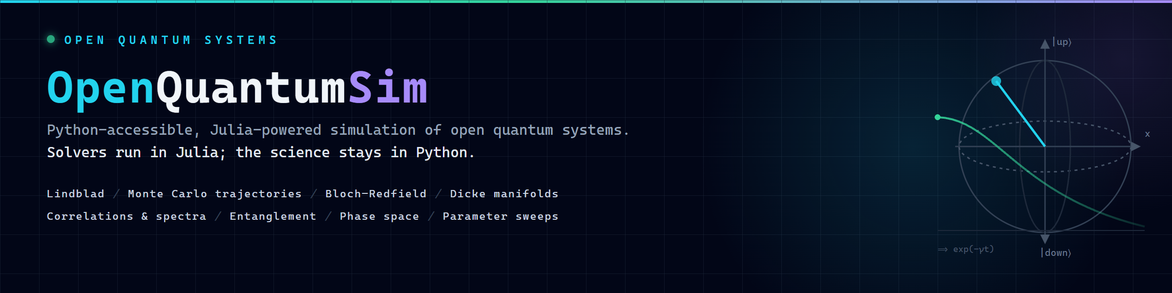
QuTiP is excellent general-purpose quantum dynamics software. OpenQuantumSim is for researchers who want a Python interface while moving expensive open-system propagation into a Julia backend: Lindblad solvers, Monte Carlo wave-function trajectories, Bloch-Redfield weak-coupling dynamics, Dicke-space collective spins, restartable parameter sweeps, HDF5 outputs, phase-space tools, and state diagnostics in one package.
- One import, no glue code.
import openquantumsim as oqsgives the full API: spaces, operators, solvers, diagnostics, plotting, and persistence. - Julia speed, Python ergonomics. Propagation runs in the packaged
OpenQuantumSimJLbackend; arrays go in, named results come back. - Validated, not just benchmarked. Analytic limits and QuTiP reference models are checked in CI on Linux and Windows.
How It Fits Together
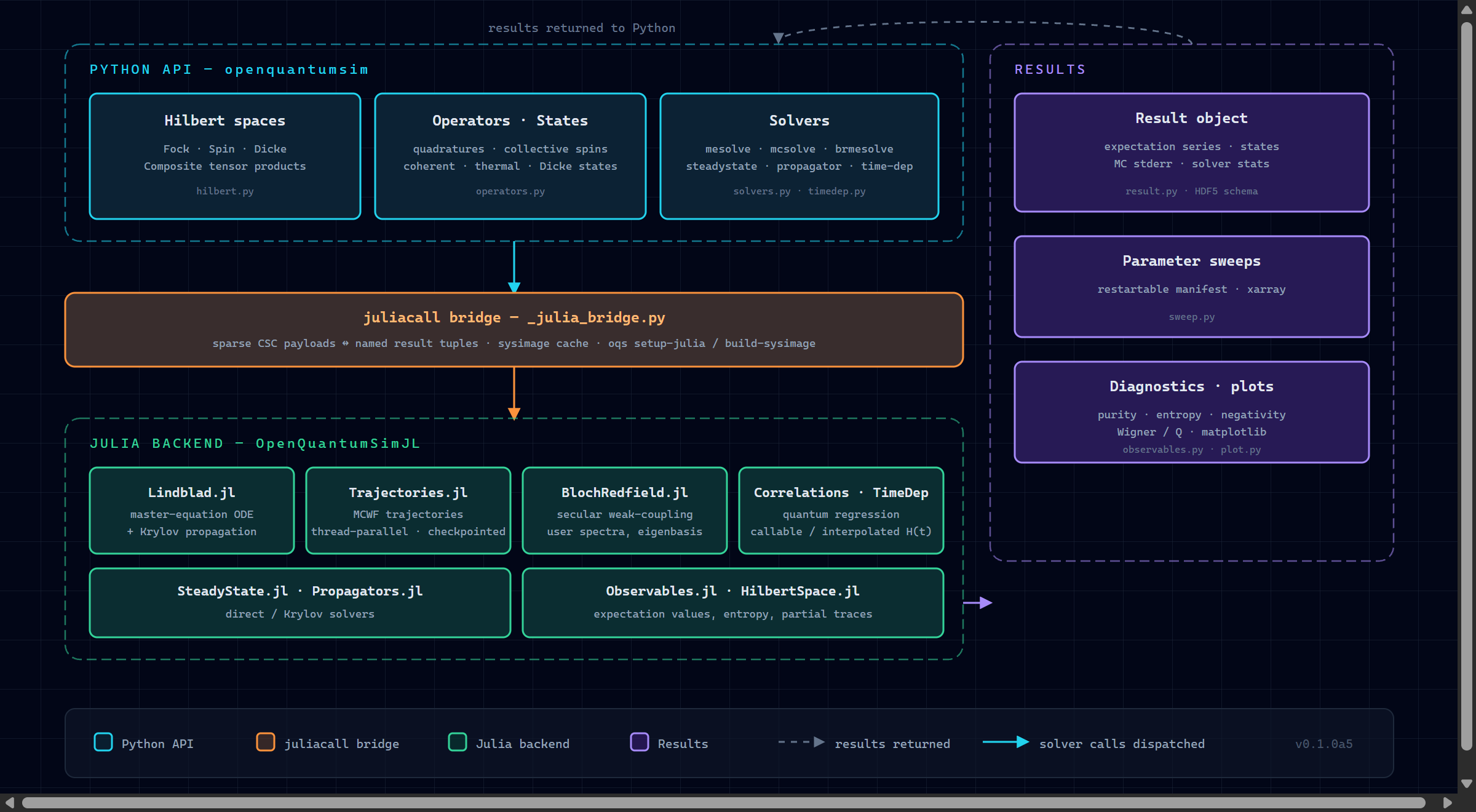
The Python API builds Hilbert spaces, operators, and solver calls. The
juliacall bridge dispatches sparse payloads to the packaged Julia backend,
where the heavy propagation runs (thread-parallel for trajectories). Named
result tuples flow back into a Result object with HDF5 persistence, xarray
sweep summaries, and matplotlib plotting on the Python side.
Performance
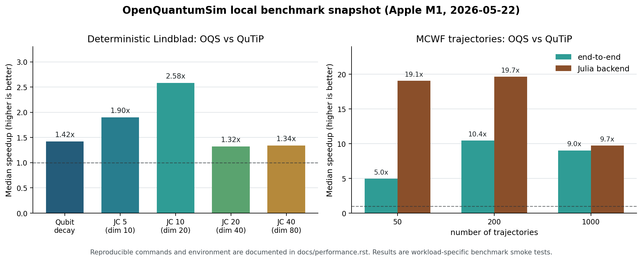
On the current Apple M1 benchmark snapshot, OpenQuantumSim is 1.3x-2.6x faster than QuTiP on deterministic Lindblad reference cases up to Hilbert dimension 80. For a qubit MCWF trajectory scaling smoke test, OpenQuantumSim is 5.0x-10.4x faster end-to-end than QuTiP, with 9.7x-19.7x faster Julia backend trajectory aggregation when using four Julia threads. The benchmark commands and environment are documented so these numbers can be reproduced and challenged.
Documentation: https://mohammadjafariph.github.io/OpenQuantumSimulation/
The package is currently released as an alpha. The API is usable, tested, and
published on PyPI, but minor interface changes may still occur before a stable
0.1 release.
Stability and the Road to 0.1.0
The core solver entry points (mesolve, mcsolve, brmesolve,
single_trajectory, steadystate, propagator), the Result object, and the
HDF5 result schema are stable-in-practice: the validation suite and CI guard
them, and no breaking change will land in a patch-level alpha release. Before
the stable 0.1.0 tag, any breaking change to a documented public function
will be announced with a deprecation warning and a changelog entry in the
preceding release.
The remaining pre-0.1.0 work (API review items and the stability date) is
tracked in the repository roadmap issue:
https://github.com/mohammadjafariph/OpenQuantumSimulation/issues
Installation
python -m pip install openquantumsim
OpenQuantumSim uses JuliaCall to load the packaged Julia backend. The first solver call on a new machine may spend a few minutes resolving and precompiling Julia packages. To make that cost explicit, run the backend setup once after installing:
oqs setup-julia
For repeated simulations, build a local Julia sysimage. This can take several minutes once. The command validates the generated image with JuliaCall before registering it, and future solver calls automatically reuse it:
oqs build-sysimage
Set OPENQUANTUMSIM_USE_SYSIMAGE=0 to temporarily disable the cached sysimage,
or OPENQUANTUMSIM_JULIA_SYSIMAGE=/path/to/sysimage to use a custom image.
Rebuild the sysimage after upgrading Julia or OpenQuantumSim.
For development from source:
git clone https://github.com/mohammadjafariph/OpenQuantumSimulation.git
cd OpenQuantumSimulation
python -m pip install -e ".[dev]"
oqs setup-julia
Features
- Hilbert-space helpers for finite Fock spaces, spin spaces, tensor-product systems, and symmetric Dicke manifolds.
- State and operator constructors for common open-system models.
- Lindblad master-equation propagation with dense and sparse backends.
- Monte Carlo wave-function trajectories with backend-side aggregation for selected diagnostics.
- Secular Bloch-Redfield dynamics with user-supplied bath spectra.
- Time-dependent Hamiltonians with callable or interpolated coefficients.
- Steady-state solves, two-time correlations, FFT spectra, and parameter sweeps.
- Propagators: unitary evolution and Lindblad superoperators for time-independent systems.
- State metrics including purity, entropy, fidelity, trace distance, populations, coherences, and Bloch-vector components.
- Entanglement diagnostics: negativity, logarithmic negativity, and two-qubit concurrence, plus mutual information on arbitrary cuts.
- Wigner and Husimi-Q phase-space distributions for finite Fock spaces.
- HDF5 result persistence for solver outputs and sweep summaries.
- Validation scripts comparing analytic limits and QuTiP reference models.
Quick Example
The example below solves spontaneous emission for a two-level system and
compares the excited-state population with the analytic result
exp(-gamma * t).
import numpy as np
import openquantumsim as oqs

atom = oqs.SpinSpace(0.5, label="atom")
excited = oqs.basis(atom, "up")

gamma = 0.2
H = 0.0 * oqs.sigmaz(atom)
rho0 = oqs.ket2dm(excited)
collapse = np.sqrt(gamma) * oqs.sigmam(atom)
projector = oqs.Operator(oqs.ket2dm(excited), atom, "P_excited")
times = np.linspace(0.0, 0.2, 3)

result = oqs.mesolve(
    H,
    rho0,
    times,
    c_ops=[collapse],
    e_ops=[projector],
    options=oqs.Options(rtol=1e-8, atol=1e-10),
)

expected = np.exp(-gamma * times)
assert np.allclose(result.expect[0].real, expected, atol=2e-7)
print(result.expect[0].real)
More complete scripts are available under examples/gallery/, including
deterministic decay, a time-dependent driven qubit, Jaynes-Cummings dynamics,
Monte Carlo trajectories, phase-space plots, restartable parameter sweeps, and
coupled-qubit entanglement dynamics with emission spectra.
Each one supports a quick smoke run:
python examples/gallery/qubit_decay.py --fast
python examples/gallery/phase_space.py --fast
Tutorial notebooks are available in the documentation, including qubit decay, Dicke synchronization, parameter sweeps, phase-space plots, and state metrics:
Time-Dependent Hamiltonians
Time-dependent systems can be written as
H(t) = H0 + sum_i f_i(t) H_i.
drive = oqs.InterpolatedCoefficient([0.0, 5.0], [0.0, 0.2])
H_t = oqs.time_dependent_hamiltonian(
    0.5 * oqs.sigmaz(atom),
    [(oqs.sigmax(atom), drive)],
)

result = oqs.mesolve(H_t, rho0, np.linspace(0.0, 5.0, 101), c_ops=[collapse])
Monte Carlo Trajectories
result = oqs.mcsolve(
    H,
    excited,
    times,
    c_ops=[collapse],
    e_ops=[projector],
    n_traj=1000,
    options=oqs.Options(seed=2026, max_step=0.01, progress=True),
)

population_mean = result.expect[0].real
population_stderr = result.expect_stderr[0].real
Long trajectory runs can checkpoint partial sums and resume from the same operators, seed, time grid, and solver options:
result = oqs.mcsolve(
    H,
    excited,
    times,
    c_ops=[collapse],
    e_ops=[projector],
    n_traj=20_000,
    options=oqs.Options(
        seed=2026,
        max_step=0.01,
        checkpoint_file="runs/mcsolve_checkpoint.h5",
        checkpoint_every=100,
    ),
)
Bloch-Redfield Dynamics
Weak system-bath coupling can be modeled with the secular Bloch-Redfield equation. Each coupling operator is paired with a spectrum callable giving the dissipator weight at a Bohr frequency; decay channels sit at negative frequencies.
kappa = 0.4
zero_temperature = lambda omega: kappa if omega < 0 else 0.0

result = oqs.brmesolve(
    H,
    rho0,
    times,
    a_ops=[(oqs.sigmam(atom), zero_temperature)],
    e_ops=[projector],
)
A constant spectrum gamma = g is equivalent to a Lindblad collapse operator
sqrt(g) * A, which makes BR results easy to sanity-check against mesolve.
State Diagnostics
State diagnostics can be evaluated during deterministic solves, single trajectories, and supported trajectory aggregations.
metrics = oqs.state_metrics(
    purity=True,
    fidelity_to=excited,
    population_indices=[0, 1],
)

trajectory = oqs.single_trajectory(
    H,
    excited,
    times,
    c_ops=[collapse],
    state_observables=metrics,
    options=oqs.Options(seed=2026, max_step=0.01),
)

purity = trajectory.state_observables["purity"].real
Parameter Sweeps
ParameterSweep expands a parameter grid, skips completed points on rerun,
writes a restartable manifest, and saves aggregate summaries.
sweep = oqs.ParameterSweep(
    base_system={"model": "qubit_decay"},
    params={"gamma": [0.05, 0.1, 0.2]},
)

run = sweep.run(run_one_point, output_dir="runs/gamma_sweep")
print(run.summary)
Phase-Space Utilities
Finite Fock-space states can be inspected with Wigner and Husimi-Q distributions.
space = oqs.FockSpace(30)
rho = oqs.ket2dm(oqs.coherent(space, 1.0 + 0.5j))
x, p = oqs.phase_space_grid(xlim=(-5.0, 5.0), points=201)

W = oqs.wigner(rho, x, p)
Q = oqs.q_function(rho, x, p)
ax = oqs.plot_wigner(rho, x, p)
Result Persistence
Solver results can be saved and loaded in HDF5 format.
result.save_hdf5("runs/qubit_decay.h5")
loaded = oqs.load_result("runs/qubit_decay.h5")
The schema stores time points, expectation series, optional saved states, state-observable series, Monte Carlo uncertainty estimates, entropy, and solver statistics.
Validation
The validation suite includes analytic qubit decay and a damped Jaynes-Cummings comparison against QuTiP.
python -m pip install -e ".[validation]"
python scripts/validate_jaynes_cummings_qutip.py
Performance comparison scripts are available under benchmarks/. Benchmark
results depend strongly on problem size, backend warmup, hardware, and thread
configuration; record those settings with any reported timings.
Documentation
Build the local documentation with:
python -m pip install -e ".[docs]"
sphinx-build -b html docs docs/_build/html
The documentation includes API pages, tutorials, validation examples, benchmark notes, and the HDF5 result schema.
Development
Run the Python test suite:
python -m pytest
Run the Julia backend tests:
julia --project=src/OpenQuantumSimJL -e 'using Pkg; Pkg.test()'
Repository layout:
openquantumsim/             Python frontend
src/OpenQuantumSimJL/       Julia backend package
tests/                      Python test suite
docs/                       Sphinx documentation
benchmarks/                 Benchmark scripts
scripts/                    Development and validation helpers
examples/                   Domain examples built on the public API
Authorship
The research idea, overall architecture and design, and the original seed Julia codes and scripts are the author's own work. Language models (LLMs) assisted with later improvements, optimizations, and porting; the author reviewed, tested, and validated the resulting code. The validation suite, benchmarks, and CI on Linux and Windows back this process.
Citation
If you use OpenQuantumSim in your research, please cite the software release
(see CITATION.cff):
OpenQuantumSim, Mohammad Jafari, https://github.com/mohammadjafariph/OpenQuantumSimulation
License
MIT — see LICENSE.
1 maintainer

Metadata
1 maintainer
Release files for openquantumsim 0.1.0a6
For a detailed explanation of source distributions (sdists) and built distributions (wheels), please see the package formats documentation.
Source distribution (sdist)
| File | Size | Uploaded | |
|---|---|---|---|
| openquantumsim-0.1.0a6.tar.gz | 100.0 kB | Details |
Built distribution (wheel)
| File | Interpreter | ABI | Platform | Reset |
|---|---|---|---|---|
| openquantumsim-0.1.0a6-py3-none-any.whl | Python 3 | none | any | Details |
Total release size: 188.8 kB
Release files / openquantumsim-0.1.0a6.tar.gz
| Download URL | openquantumsim-0.1.0a6.tar.gz |
|---|---|
| Size | 100.0 kB |
| Tags | Source |
|
SHA-256 checksum How to use checksums |
b80ff5505d7ec0f59df86531f0014c98f3cc68f3ad9be816b9b3cb01153ed73d
|
|
BLAKE2b-256 checksum How to use checksums |
3d309991ecf4c0236714bba0ec38e1e5dbcee07879f8771e16b0e55fac37e475
|
| Upload date | |
|
Uploaded using Trusted Publishing? What is trusted publishing? |
Yes |
| Uploaded via |
twine/7.0.0 CPython/3.13.14
|
Provenance
Provenance describes where a file came from. On PyPI, provenance is shared via attestations, which provide a verifiable record of the build or publishing details. View details, limitations and caveats.


PyPI Publish Attestation
PyPI verified that this artifact, at this checksum, originated from the publisher listed below.
Signed by GitHub Actions, verified by PyPI on Sep 30, 2026.
Transparency logRelease files / openquantumsim-0.1.0a6-py3-none-any.whl
| Download URL | openquantumsim-0.1.0a6-py3-none-any.whl |
|---|---|
| Size | 88.8 kB |
| Tags | Python 3 |
|
SHA-256 checksum How to use checksums |
a2cc16cfc2da9cf778c592091d4f727559a4a518379eca66d289c7ee01e5dbed
|
|
BLAKE2b-256 checksum How to use checksums |
c37e340c608f8c1d12fa22d450bfe5e1d99dbc7ec626d1b5a3cba43bf43f1416
|
| Upload date | |
|
Uploaded using Trusted Publishing? What is trusted publishing? |
Yes |
| Uploaded via |
twine/7.0.0 CPython/3.13.14
|
Provenance
Provenance describes where a file came from. On PyPI, provenance is shared via attestations, which provide a verifiable record of the build or publishing details. View details, limitations and caveats.
PyPI Publish Attestation
PyPI verified that this artifact, at this checksum, originated from the publisher listed below.
Signed by GitHub Actions, verified by PyPI on Sep 30, 2026.
Transparency log













