




Automated quantitative DCE-MRI of cerebral perfusion, microvasculature, and blood–brain-barrier permeability. Point it at a subject's scans and it produces the full derivatives tree — T1/M0 mapping, arterial-input-function extraction, signal-to-concentration, and pharmacokinetic and diffusion modelling — as voxel-, tissue-, and parcel-level maps. No notebook, GUI, or server.
Install · Quickstart · Example run · How it works · Data layouts · Commands · Assist · Configuration · Principles · Citation

p-Brain (the p is for perfusion and permeability) is a
cross-platform command-line tool for quantitative DCE-MRI. It serves two
purposes. As shipped, it is a validated, ready-to-run pipeline you point at real
scanner data to get quantitative maps (Ki, CBF, MTT, CTH, Ktrans, FA, and
others). It is also a framework you extend: each step — kinetic model, AIF,
segmentation backend, or a whole stage — is a self-contained plug-in, so adding
your own means writing a single file with no changes to the core. Drop a model
into pbrain/models/, call it with --models yourmodel, and it runs on every
subject, is aggregated to every anatomical level, is written as NIfTI/CSV/JSON,
and is given diagnostics automatically.
 Install
pip install p-brain
pbrain --help
Optional extras pull in heavier dependencies only when you need them:
pip install "p-brain[cnn]"        # TensorFlow — the CNN arterial-input-function (default AIF)
pip install "p-brain[metal]"      # Apple-Silicon GPU for the TF stages (pins TF 2.16 + tensorflow-metal)
pip install "p-brain[diffusion]"  # dipy — the diffusion track (DTI, DKI, CSD, tractography)
pip install "p-brain[dicom]"      # pydicom — DICOM input
pip install "p-brain[all]"        # everything at once
On Apple Silicon, [metal] is how the CNN AIF and SynthSeg run on the GPU —
Apple's tensorflow-metal plugin only supports TensorFlow ≤ 2.16, so this pins
the matched pair. Install it into a fresh environment (a newer TensorFlow
already present can't be safely downgraded in place). On Linux, GPU works through
[cnn] with a CUDA build of TensorFlow. Without a GPU backend, --device mps/cuda
cleanly falls back to CPU (identical results, only slower).
Runs on Linux, macOS, and Windows with Python 3.10–3.12. From a clone,
pip install -e ".[dev]" installs it in editable mode.
Quickstart
pbrain setup            # interactive: install extras, offer to fetch weights and data
pbrain fetch-weights    # CNN weights           (Zenodo 10.5281/zenodo.15697443)
pbrain fetch-data       # example subject sub-01 (Zenodo 10.5281/zenodo.20826857, ~99 MB)
pbrain fetch-data downloads a real subject and prints a ready-to-run,
weights-free command. Then, on your own data:
# One flag on raw Philips PAR/REC: inputs are auto-discovered by protocol name
pbrain run --subject-dir /data/20230403x2

# A whole study: each sub-directory is a subject, run in parallel
pbrain run-cohort --cohort /data/patients /data/controls --workers 4
Example run
On an interactive terminal, pbrain run opens a live cockpit — the brain draws
itself in, then an analysis panel tracks the pipeline while log lines scroll
above it and a status line shows where it is:
  ⢀⣴⣿⣿⣿⣷⣦⡀
  ⠈⢻⣿⣿⣿⣿⣿⠿   p-Brain
  ⠀⠀⠉⠉⠹⣿⠟⠀   perfusion & permeability

  reading DCE … dcm2niix
  DCE shape · 256×256×10 · 250 frames
  fitting T1 map … median 1642 ms
╭──────────────────────── analysis ────────────────────────╮
│  ✓ load            DCE 256×256×10·250, IR 8 TIs           │
│  ✓ t1_m0           T1 median 1642 ms                      │
│  ✓ signal_to_conc  saturation_recovery                    │
│  ◆ aif             extracting … ROI 704 vox · peak 3.2 mM │
│  ○ tissue_roi      synthseg                               │
│  ○ kinetic         patlak · tikhonov                      │
╰───────────────────────────────────────────────────────────╯
 ⠴ p-Brain · aif · 22s · CNN rICA, 3 slices        auto ⇥
Piped or redirected (| tee, > log, --quiet), the cockpit is suppressed and
you get plain, greppable log lines instead — the numeric results are identical
either way.
How it works
Ten self-contained stages, each cached to the derivatives tree and re-runnable in isolation:
 load ──▶ t1_m0 ──▶ signal_to_conc ──▶ aif ──▶ tissue_roi ──▶ normalisation
   │      (T1/M0)   (signal → mM)     (CNN /   (SynthSeg      (baseline,
   │                                   auto)    parcels)       Gd leak)
   ▼
 kinetic ──▶ diffusion ──▶ summary ──▶ diagnostics
 (patlak,    (DTI/DKI/     (voxel ·    (per-map QC
  tikhonov,   CSD, tracts)  tissue ·    overlays)
  tofts…)                   parcel)
Every stage is a plug-in resolved at run time; pbrain list shows all
plug-points, pbrain list models drills into one. Results are written at three
levels (voxel, tissue-region, parcel) in NIfTI, CSV, and JSON, with a diagnostics
montage per map.
Inputs are normalised first. The load stage converts whatever you point it at
— Philips PAR/REC or DICOM (via dcm2niix), NIfTI passed straight through — into the
4-D NIfTI the rest of the pipeline runs on. Every downstream stage sees the same
canonical volume, so the analysis is source-format-agnostic.
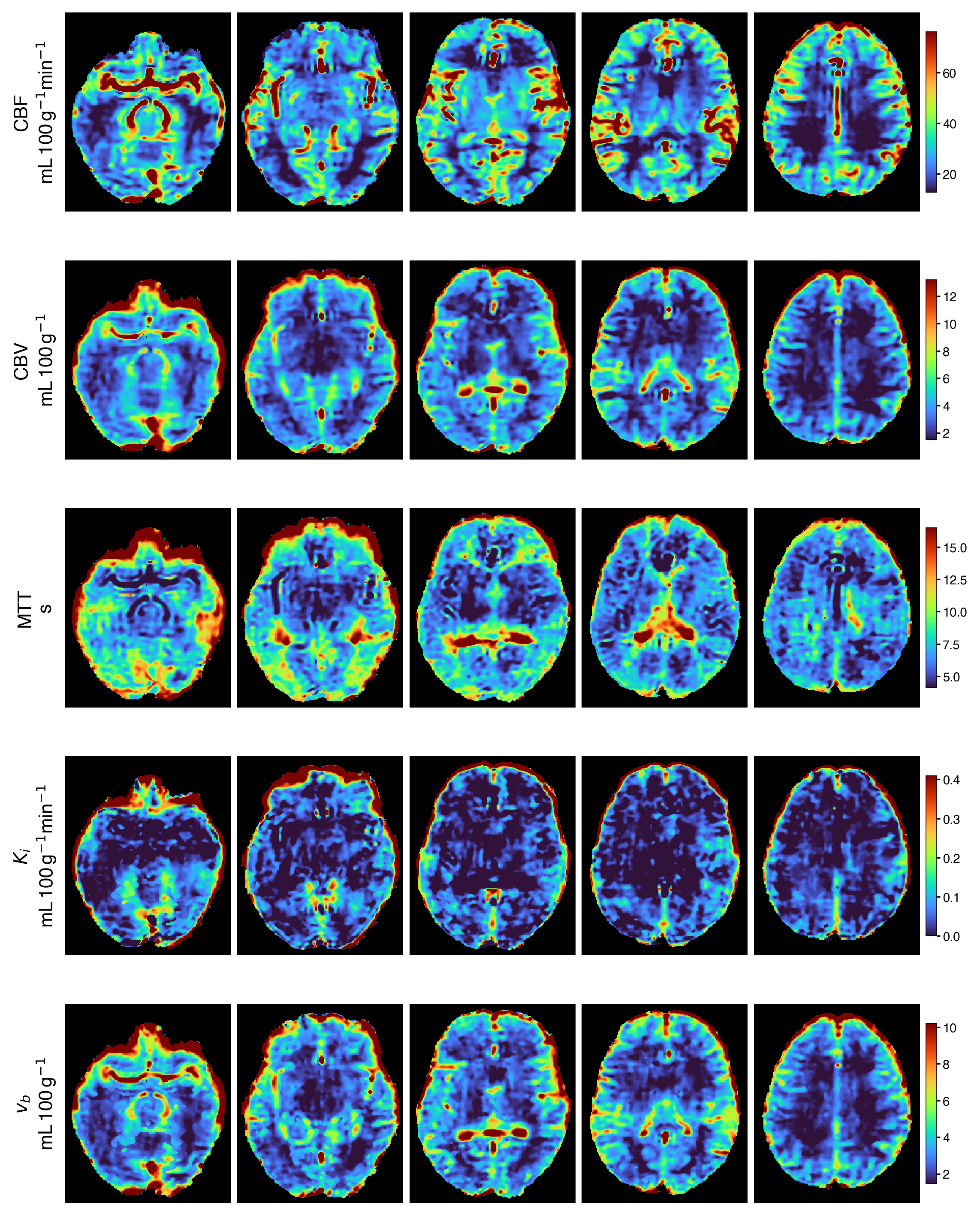
Voxelwise Ki, vb, CBF, MTT and CBV from a single automated pbrain run.
Data layouts
pbrain run <path> works out what you pointed it at — one subject or a whole
folder — and which on-disk convention it follows, then runs accordingly:
pbrain run /data/20230403x2        # one subject → runs it
pbrain run /data/patients          # a folder of subjects → fans out as a cohort
pbrain layout /data/patients       # preview what it detects (read-only, no run)
Three layouts are recognised out of the box:
| layout | a subject looks like | inputs resolved from |
|---|---|---|
| PAR/REC | Philips *.PAR with an hperf* DCE |
protocol names |
| flat-NIfTI | dce.nii.gz (+ optional t1, ir) |
file names |
| BIDS | dataset_description.json · sub-* · anat/*_T1w |
BIDS entities |
Detection is deterministic and tries single-subject first, so a subject you've
already run once (it has a pbrain/ output tree) isn't read as a one-subject
cohort.
Don't know the layout, or which file is which? --assist works it out. Point
it at a folder no built-in convention recognises and a local model reads the file
tree — names only, no pixel data — to propose which folders are subjects and
which files are the DCE, T1, and IR. You accept the proposal or correct it in
plain words ("the T1 is the MP-RAGE, not the FLAIR"). The confirmed layout is
frozen to pbrain.layout.toml at the data root, so later runs read it directly
— point-at-anything convenience with a reproducible pipeline. More in
Assist.
Commands
| command | description |
|---|---|
pbrain run <path> |
run one subject, or a folder of them — auto-detected |
pbrain layout <path> |
preview the detected layout (subject vs cohort, inputs) |
pbrain cohort --cohort A B |
run a study explicitly, in parallel (--workers N) |
pbrain plan … |
show the resolved pipeline plan without computing |
pbrain list [models|aif|…] |
all plug-points, or one in detail |
pbrain setup |
detect tooling, install extras, fetch weights/data |
pbrain fetch-weights · fetch-data |
download the CNN weights · the example subject |
pbrain methods --subject-dir X |
draft a Methods paragraph from a run's provenance |
pbrain assist |
set up the optional local model backend (Ollama) |
pbrain theme <name> · tone <n> |
banner/log palette · one-, two-, or three-tone brain |
pbrain check-deps |
verify the numeric core and report optional extras |
Assist
Running a subject usually means knowing which series is the DCE, which is the T1,
where the IR sits, and how your folders are arranged. --assist lifts that
requirement — an optional local-model layer that reads your acquisition
parameters and file tree and proposes the mapping, so you can run a subject, or a
whole unfamiliar archive, without hand-writing a single path.
pbrain run --subject-dir X --assist
What it does:
- Finds your inputs for you. From the scan headers it proposes which series is
the DCE, T1, and IR; for a folder no built-in layout recognises, it reads the
file tree (names only) and proposes which folders are subjects and which files
are each input. You accept it, or correct it in plain words — "the T1 is the
MP-RAGE" — and it re-proposes. A confirmed layout is frozen to
pbrain.layout.toml, so later runs read it directly. - Explains a failure. When a stage errors, it turns the traceback into a plain-language cause and a concrete fix.
- Writes the boilerplate. It summarises each stage's QC in a sentence and drafts a Methods paragraph from the run's provenance, ready to edit for a paper.
Two things keep it safe to leave on:
- It reads text, not data. The model sees scan headers, run provenance, QC statistics, and error messages — not voxel values — and it computes no result. The maps come from the deterministic pipeline. A suggestion that would change a run, such as which series is the DCE, takes effect only after you confirm it, and is written to the manifest so a re-run reproduces the same numbers.
- It's local and opt-in. Assist talks only to a model running on your machine via Ollama. With none configured, the assist features stay off and the run is unchanged. First use walks you through installing Ollama and pulling a model sized to your hardware, and asks before it downloads anything.
Live controls
During an interactive run:
-
Review mode.
--mode auto(default) runs straight through.--mode verifyopens a browser review at each decision checkpoint so you can confirm the suggested choice;--mode manualadditionally lets you correct it. The checkpoints:- AIF — the input-function curve and its vessel ROI on the DCE slice (with a motion-correction toggle and the candidate vessels); confirm, drag the max voxel, or draw the ROI yourself.
- Baseline — the pre-contrast baseline point on the first-peak region of the mean curve; confirm or drag it.
- Tissue segmentation — the parcellation mask across slices; confirm, or draw exclusion regions to cut artefacts out of the tissue mask.
- Per kinetic model — the model's own plot (Patlak plot; tissue-curve fit for
the residue/compartment models) with its parameter values. In manual mode some
models expose editable fit parameters (e.g. Patlak's fit-window and regression)
that re-fit live on confirm. Any model gains a review for free by defining
review(). - Diffusion — a scalar-map summary (median FA/MD/… + the primary map's central slice) for every diffusion model.
Reject any review to stop the run; ⇥ Tab cycles the mode live, shown in the status line, and the run timers pause while a review is open. Everything is served locally (no data leaves your machine) and your choice is recorded in the manifest, so a re-run reproduces it.
-
Ctrl-C stops cleanly at any point; completed stages are cached, so the next run picks up where it left off.
Configuration
Flags override a config file, which overrides defaults.
pbrain run --config study.toml --subject-dir X
pbrain run --subject-dir X --models patlak,tikhonov --opt models.patlak.regression=ols
--config takes TOML (built-in) or YAML (pip install pyyaml). Any plug-in
option is settable with --opt <plugin>.<key>.<opt>=<value> or in the file.
Acquisition parameters (flip angle, TR) are read from the scan sidecar when
present and can be overridden per run.
Add your own
Every plug-point (kinetic models, AIF extractors, signal-to-concentration,
segmentation backends, diffusion models, whole stages) is a single file that
registers itself. A kinetic model is a dataclass declaring what it accepts,
what it produces, and an extract/fit method:
# pbrain/models/my_model.py — then: pbrain run --models my_model
@dataclass(frozen=True, slots=True)
class MyModel:
    key = "my_model"
    produces = {"ki_map": np.ndarray}
    def fit(self, conc, aif, t_s, **opts) -> dict: ...
It is then aggregated to every level, written in every format, and given diagnostics with no further wiring.
Models
Set any option with --opt models.<key>.<opt>=<value>. Defaults are what you get
without setting anything.
| model | produces | notes |
|---|---|---|
patlak |
Ki, vp | Patlak graphical analysis; robust Huber slope, smart tail detection |
tikhonov |
CBF, MTT, CTH | regularised residue deconvolution; GCV / L-curve / evidence λ selection |
extended_tofts |
Ktrans, ve, vp, kep | constrained Levenberg–Marquardt; no tuning for the default fit |
The list is meant to be extended — see Add your own. The
diffusion track (--diffusion) adds FA, MD, and tractography via dipy.
Principles

--assist-resolved layout is written to pbrain.layout.toml. The same inputs and settings produce the same outputs.
load converts PAR/REC, DICOM, or NIfTI to a 4-D NIfTI; every downstream stage operates on that volume.
--quiet run emits plain text with identical numeric results.
Requirements
- Linux, macOS, or Windows with Python 3.10–3.12
dcm2niixon PATH for PAR/REC and DICOM conversion- Optional: TensorFlow (
[cnn]), dipy ([diffusion]), Ollama (assist)
Citation
If p-Brain contributes to your work, please cite the accompanying paper (Tireli
et al.) and this repository. See
LICENSE for terms.
MIT · Built by Edis Devin Tireli · Functional Imaging Unit, Rigshospitalet · University of Copenhagen
1 maintainer

Download files
Download the file for your platform. If you're not sure which to choose, learn more about installing packages.
Source Distribution
Built Distribution
Filter files by name, interpreter, ABI, and platform.
If you're not sure about the file name format, learn more about wheel file names.
Copy a direct link to the current filters
File details
Details for the file p_brain-3.1.2.tar.gz.
File metadata
- Download URL: p_brain-3.1.2.tar.gz
- Upload date:
- Size: 375.6 kB
- Tags: Source
- Uploaded using Trusted Publishing? No
- Uploaded via:
uv/0.5.9
File hashes
| Algorithm | Hash digest | |
|---|---|---|
| SHA256 |
b9ea5bfeb657640eff27ed0187c7c635f9b7228cc45bd3e52e573ba6952492cf
|
|
| MD5 |
9fade8c5eb73de151f02edfb46da2e57
|
|
| BLAKE2b-256 |
3708078231153d29aa249e24db6b541639cae7fba6c1e6d2fe50df4a6fb7d6c6
|
File details
Details for the file p_brain-3.1.2-py3-none-any.whl.
File metadata
- Download URL: p_brain-3.1.2-py3-none-any.whl
- Upload date:
- Size: 419.6 kB
- Tags: Python 3
- Uploaded using Trusted Publishing? No
- Uploaded via:
uv/0.5.9
File hashes
| Algorithm | Hash digest | |
|---|---|---|
| SHA256 |
cd16398e1c010b5739f1d3a5cbd40e46d177d1d7dc610e8c25efc0a6dc9410a3
|
|
| MD5 |
f9ab280a46e4d36e15302e864dfa259d
|
|
| BLAKE2b-256 |
8ad9c2141ec9d8b0ae1bea60616f96584bc675ccc912f92d45f79e30b7d909d5
|














