
ppgrid - Pull-Push Scattered-Data Interpolation


Fast, continent-scale raster interpolation for scattered point data. Turns tens of millions of geolocated points into a pair of GeoTIFFs in minutes on a single machine. No GPU needed.
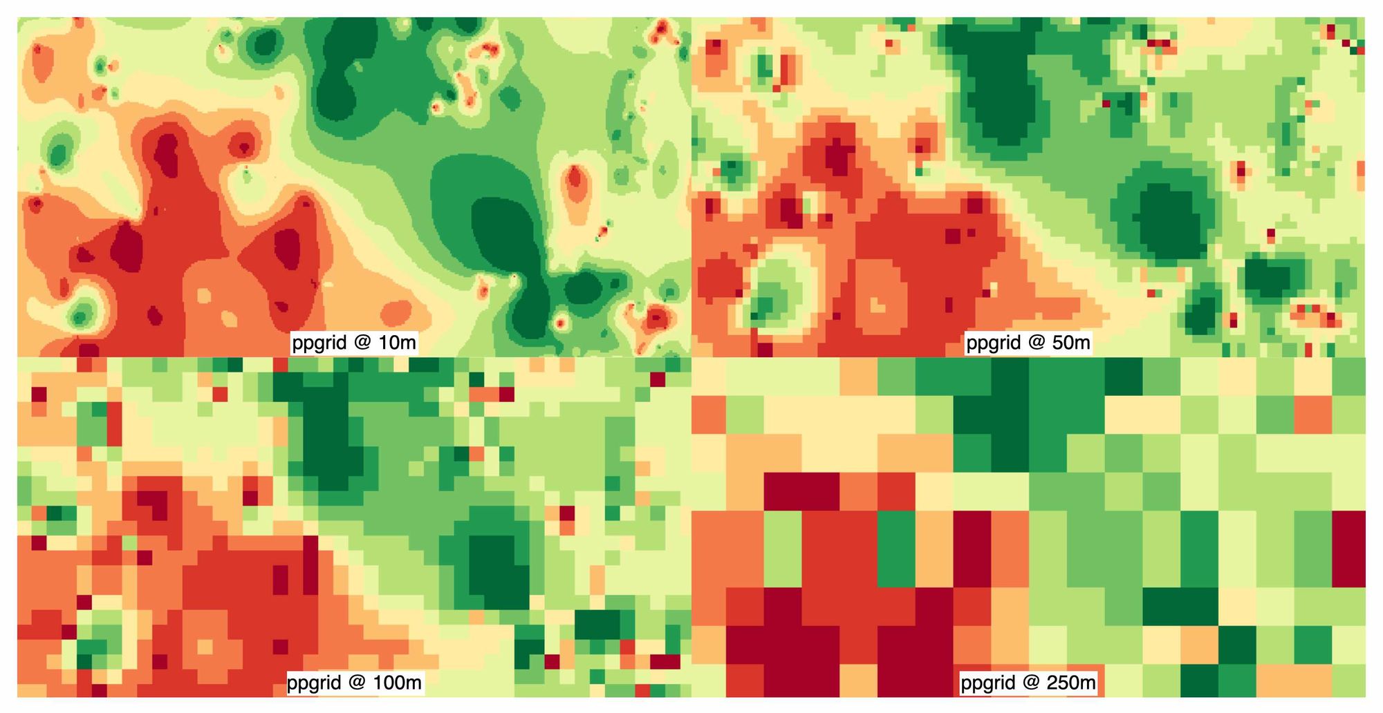
A single 100K-point dataset rendered at four resolutions. The adaptive mipmap pyramid fills sparse regions from coarser layers, so you get a continuous surface instead of patchy gaps.
What it does
You have N points with (longitude, latitude, value). You want a raster where every cell within a specified distance of real data carries an interpolated value, and everything else is nodata.
Standard IDW in QGIS or ArcGIS is O(N*M) (hours to days at 16M points, depending on the IDW implementation and machine). This tool uses pull-push mipmap interpolation to reduce cost to O(M), independent of N.
How it works
Pull-Push (mipmap) Interpolation
Based on Gortler et al. 1996 (Lumigraph) and Kraus 2009.
Once points are snapped to a grid, IDW is exactly a normalised convolution:
z = (S ⊛ K) / (C ⊛ K) K(r) = r^-p
Pull-push evaluates this across a mipmap pyramid so cost is O(M), independent of N.
Steps:
- Points are binned into
S(sum of transformed values) andC(count) grids - A mipmap pyramid is built by repeated 2x2 block sums
- The coarsest level seeds the interpolation
- Descending the pyramid, each level blends local estimate vs upsampled parent
- Local confidence is
min(C/saturation, 1). Dense cells trust themselves, sparse cells inherit - A summed-area table (
box_count) provides an exact radius fill cap
Output bands:
- Value: int16, 0-100 percentile,
percentile = DN/scale - Support km: int16,
support_km = 2^(DN/8), effective spatial scale of estimate
Working CRS: EPSG:6933 (Wagner VII) by default. Global equal-area, metres are true. Configurable via --work-crs.
Output CRS: EPSG:3857 (Web Mercator) by default. Configurable via --out-crs.
Calibration (optional)
Before interpolation, the tool can:
- Choose a transform. Tests identity/log10/sqrt/percentile and picks the one with highest intraclass correlation across coarse scales
- Derive a fill cap. Spatially blocked cross-validation to find the honest distance beyond which interpolation has no skill
- Save calibration.json. Contains the percentile-to-value lookup table for decoding the output raster back to real units
Install
Requires Python 3.11+ (older interpreters fail the pip resolver with a bare error).
pip install ppgrid
For Parquet support:
pip install ppgrid[parquet]
Or from source:
git clone https://github.com/marzukia/ppgrid.git
cd ppgrid
uv sync
Quick Start
ppgrid data.csv --value-col price --res 500 --cap-km 10 --skip-calibration
This reads data.csv, interpolates the price column at 500m resolution with a 10km fill cap, and writes value.tif + support_km.tif to out/.
Usage
# Quick run (skip calibration)
ppgrid data.csv --value-col premium --res 500 --cap-km 64 --skip-calibration

# Full run with calibration (saves calibration.json)
ppgrid data.csv --value-col premium --res 100 --cap-km auto

# Custom projection and params
ppgrid data.csv --value-col premium --res 100 --cap-km 25 --transform log10 --workers 8

# Reuse existing calibration
ppgrid data.csv --value-col premium --calibration calibration.json

# Round output percentiles to a step (e.g. 5 -> 90/95/100) for clean vectorisation
ppgrid data.csv --value-col premium --res 100 --cap-km 25 --percentile-step 5

# Print help with examples (also: --help)
ppgrid help
CLI Options
| Flag | Default | Description |
|---|---|---|
input |
— | CSV or Parquet input path (bare ppgrid exits 2 with a hint; ppgrid help prints usage) |
-o, --out |
out/ |
Output directory |
--value-col |
value |
Value column name |
--lng-col |
longitude |
Longitude column name |
--lat-col |
latitude |
Latitude column name |
--res |
500.0 |
Cell size in metres |
--cap-km |
auto |
Fill cap km, or 'auto' (blocked-CV derived) |
--transform |
auto |
auto, identity, log10, sqrt, percentile |
--saturation |
1.0 |
Counts for a cell to fully self-trust |
--block |
2048 |
Block size in cells |
--workers |
4 |
Number of parallel workers |
--scale |
100.0 |
DN = percentile * scale |
--percentile-step |
(none) | Round output percentiles to the nearest step (e.g. 5 -> 90/95/100) |
--compress |
ZSTD |
GeoTIFF compression |
--calibration |
(none) | Path to existing calibration.json |
--calib-max-points |
2000000 |
Max points to use for calibration |
--src-crs |
4326 |
Input coordinate reference system |
--work-crs |
6933 |
Working CRS for interpolation (equal-area) |
--out-crs |
3857 |
Output CRS for final GeoTIFF |
--skip-calibration |
False | Skip calibration, use defaults |
--turbo |
(none) | Turbo mode: multithreaded pipeline sized to a RAM cap. Optional preset `16 |
--max-ram |
(none) | Explicit RAM cap in GB (overrides the --turbo preset). Implies --turbo |
--ram-gb |
(none) | Alias of --max-ram |
--turbo-strict |
False | Shared path infeasible under the budget: error + exit 3 instead of [warn] + per-box fallback (exit 0) |
--verbose |
False | Debug logging: per-phase wall times + volumetric detail (shorthand for --log-level debug) |
--log-level |
info |
Progress log level on stderr: error, warning, info, debug (env LOGGING; verbose = debug) |
Turbo mode
--turbo enables the multithreaded pipeline. The RAM cap C (a preset, --max-ram, or bare --turbo auto-detect) drives a planning budget Bt = 0.85 * C - 4 GB and a regime, printed by a pre-check after gridding. None of the turbo settings change the output bytes.
- A — full in-RAM shared fields. Fastest; needs the most RAM.
- B — input in RAM, output bands file-backed with a limited number of descent bands in flight.
- C — shared all-memmap banded descent: input and output bands file-backed (reclaimable memmap), with an 8 GB page-cache floor in its peak accounting.
- per_box — per-box warp/write fallback, taken when regime C has fewer than 2 in-flight units. This is the only genuine low-RAM mode.
When the shared path is infeasible under the budget, the run prints [warn] and continues on the per-box path (exit 0, correct output). --turbo-strict makes the infeasibility an error (exit 3).
--ram-gb caps the shared-field budget, not process RSS. Write/descent buffers sit outside the Bt sizing, so a regime C run under --ram-gb 20 can peak well above 20 GB RSS (measured: 39.4 GB). Only the per-box path is genuinely low-RAM (measured: 8.5 GB peak).
Byte identity. Turbo output is sha256-identical to the serial path. The optional parallel per-tile ZSTD write is gated by a compression oracle: where the oracle mismatches (e.g. the reference GDAL 3.12.4 / libtiff 6.2 stack), the run uses the stock-codec parallel writer instead, which is byte-exact; the serial per-band write is the last resort only, reached if that writer's layout guards fail.
Decoding the output
The value band stores percentiles, not raw values. To convert back to real units, use the calibration.json saved in the output folder:
import json, numpy as np, rasterio

with open("calibration.json") as f:
    quantiles = np.array(json.load(f)["percentile_quantiles"])

with rasterio.open("value.tif") as r:
    percentiles = np.array(r.read(1), copy=True) / 100.0

real_values = np.interp(percentiles, np.linspace(0, 100, len(quantiles)), quantiles)
Benchmarks
Head-to-head on a 100K-point synthetic dataset (M4 MacBook Pro, 24GB) against the traditional GDAL path:
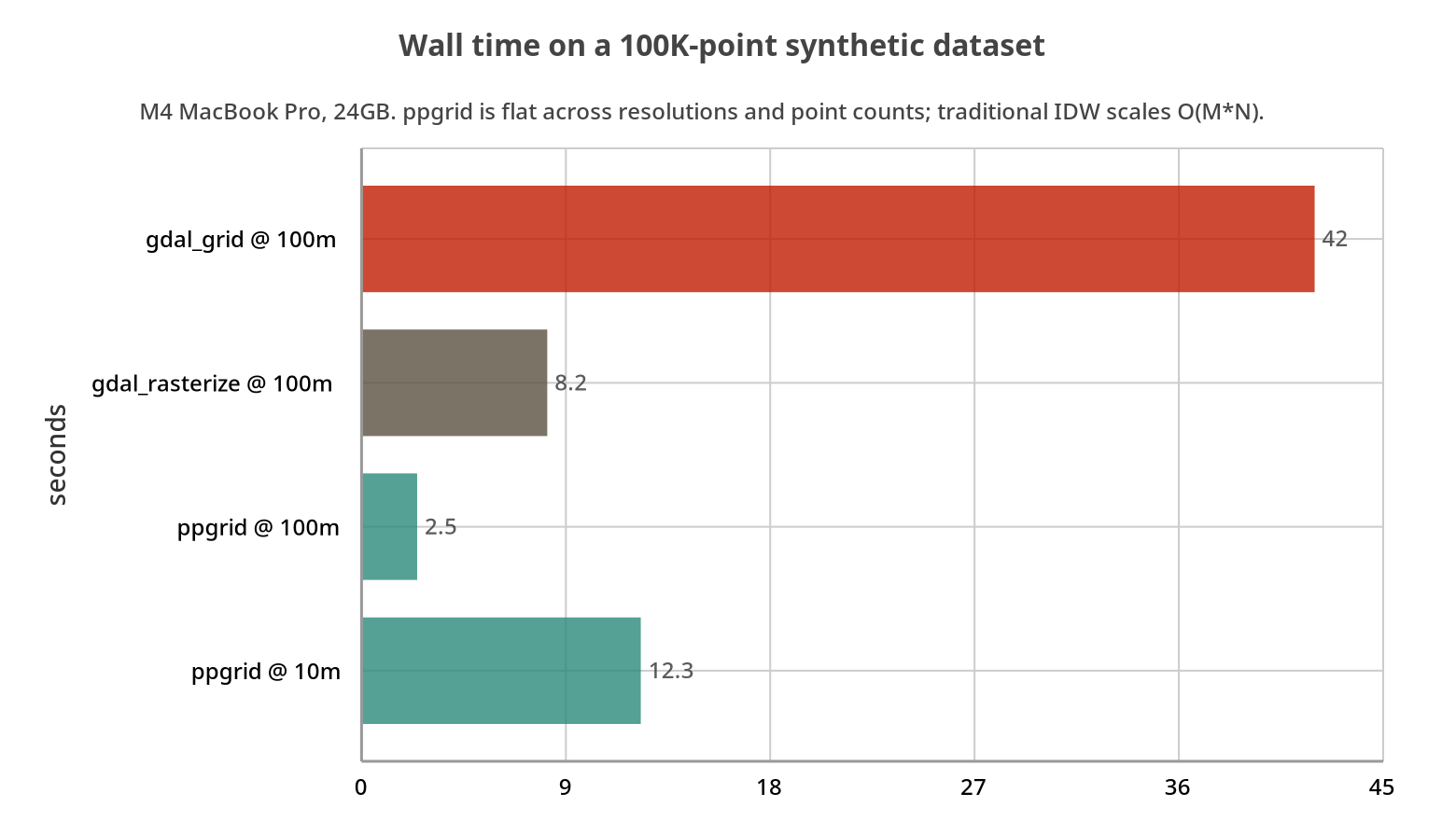
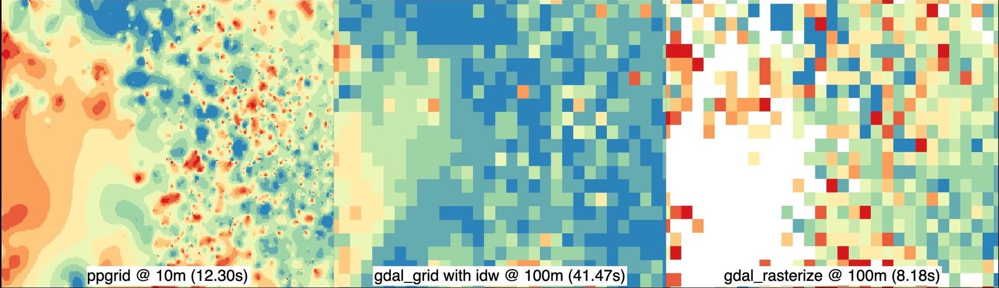
ppgrid at 100m is ~17x faster than gdal_grid and ~3x faster than gdal_rasterize at the same resolution, and it can run 10x finer (10m) in under 13 seconds.
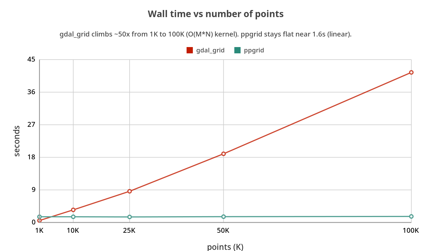
The reason is the scaling behaviour. As the point count grows, gdal_grid climbs ~50x from 1K to 100K points (the O(M*N) kernel), while ppgrid stays flat near 1.6s because each point is binned once and the rest is linear over raster cells:
Resolution sweep
Melbourne Housing dataset (13,580 points) at various resolutions on the same machine:
| Resolution | Wall Time | File Size |
|---|---|---|
| 10m | 26.6s | 27.3 MB |
| 25m | 4.0s | 6.8 MB |
| 50m | 1.3s | 2.3 MB |
| 100m | 0.8s | 749 KB |
| 250m | 0.6s | 159 KB |
| 500m | 0.6s | 49 KB |
Turbo benchmarks (full AU)
Full-Australia grid, 16M points, --res 100 --cap-km 25 --skip-calibration, on marzuki-hydrogen (Threadripper 24C/48T, 125 GB, CPU-only). All outputs sha256-identical across the pre- and post-turbo-code runs.
| Mode | Wall | Peak RSS |
|---|---|---|
Pre-PR turbo code, regime A (--turbo 64, same code) |
30:45 (quiet) to 50:46 (loaded) | 41.7 GB |
Regime A (--turbo 64) |
2:33 | 43 GB |
| per-box (24 GB cgroup slice) | 3:20 | 8.5 GB |
Regime C (--ram-gb 20) |
6:25 pre-PR, 3:08 post | 39.4 GB |
The pre-PR regime-A wall varies 30:45-50:46 with machine load (two measured runs of the same code on the same box), so the speedup range is ~12-20x rather than a single ratio. Note the --ram-gb 20 row: the cap bounds the shared-field budget, not RSS — see the caveat above; per-box is the only genuinely low-RAM mode.
Example Outputs
ppgrid against gdal_grid + IDW and gdal_rasterize on the same data. Left is ppgrid, middle is gdal_grid with IDW, right is gdal_rasterize:
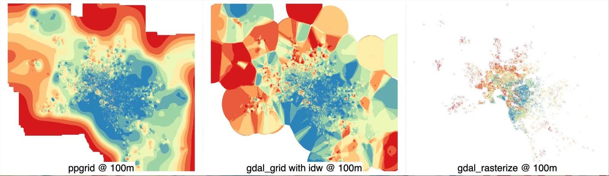
Zoomed in. ppgrid stays continuous where the grid-based methods produce Voronoi-style polygons and patchy gaps:
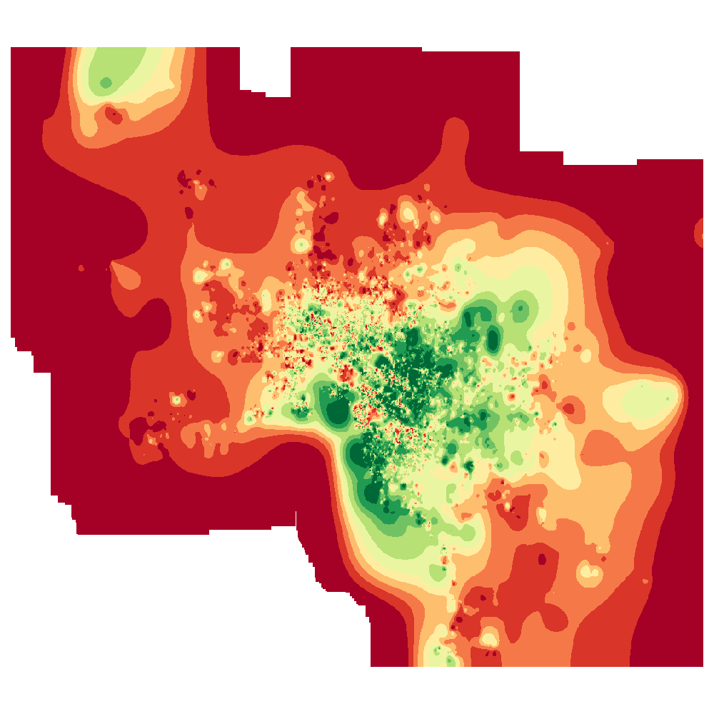
Melbourne Housing interpolated at 10m, full extent:
Data
data/melb_houses.csv: 13,580 Melbourne property sales with latitude, longitude, and price. Sourced from the Melbourne Housing Snapshot (CC BY-NC-SA 4.0).
data/all_equakes.csv: 44,376 earthquake events from Jan-Aug 2026, mag >= 1.5.
Data Lineage
| Step | Description |
|---|---|
| Source | USGS Earthquake Hazards Program |
| API | FDSN Event Web Service |
| Download | Batched CSV requests by month, minmagnitude=1.5, starttime=2026-01-01, endtime=2026-08-08 |
| Processing | Concatenated monthly CSVs (deduplicated header) into single file |
| License | Public Domain (USGS federal data) |
Columns Used
latitude/longitude: spatial coordinates (WGS 84)mag: earthquake magnitude (continuous, for interpolation)depth: focal depth in km (optional value layer)time: event timestamp (ISO 8601)
1 maintainer

Metadata
1 maintainer
Release files for ppgrid 0.4.1
For a detailed explanation of source distributions (sdists) and built distributions (wheels), please see the package formats documentation.
Source distribution (sdist)
| File | Size | Uploaded | |
|---|---|---|---|
| ppgrid-0.4.1.tar.gz | 329.6 kB | Details |
Built distribution (wheel)
| File | Interpreter | ABI | Platform | Reset |
|---|---|---|---|---|
| ppgrid-0.4.1-py3-none-any.whl | Python 3 | none | any | Details |
Total release size: 412.8 kB
Release files / ppgrid-0.4.1.tar.gz
| Download URL | ppgrid-0.4.1.tar.gz |
|---|---|
| Size | 329.6 kB |
| Tags | Source |
|
SHA-256 checksum How to use checksums |
e20fb81a136782baeba71305cf496105eb9e176a523883dea6b8a78dcda2feb4
|
|
BLAKE2b-256 checksum How to use checksums |
c82f614b534fc181eaf9a8916e281167d5f68268f7e2487205f261f8301142f9
|
| Upload date | |
|
Uploaded using Trusted Publishing? What is trusted publishing? |
No |
| Uploaded via |
uv/0.12.24 {"installer":{"name":"uv","version":"0.12.24","subcommand":["publish"]},"python":null,"implementation":{"name":null,"version":null},"distro":{"name":"Ubuntu","version":"24.04","id":"noble","libc":null},"system":{"name":null,"release":null},"cpu":null,"openssl_version":null,"setuptools_version":null,"rustc_version":null,"ci":true}
|
Release files / ppgrid-0.4.1-py3-none-any.whl
| Download URL | ppgrid-0.4.1-py3-none-any.whl |
|---|---|
| Size | 83.2 kB |
| Tags | Python 3 |
|
SHA-256 checksum How to use checksums |
4cd6911c7334ced2f363e7bf9f5a08ba8507522c8cd46542f70e6e2e40f24fe9
|
|
BLAKE2b-256 checksum How to use checksums |
bcbb3a409dc07b9342c8bd03f59f8de9b53985dc252b97aaf9f7d1cff2c6e47c
|
| Upload date | |
|
Uploaded using Trusted Publishing? What is trusted publishing? |
No |
| Uploaded via |
uv/0.12.24 {"installer":{"name":"uv","version":"0.12.24","subcommand":["publish"]},"python":null,"implementation":{"name":null,"version":null},"distro":{"name":"Ubuntu","version":"24.04","id":"noble","libc":null},"system":{"name":null,"release":null},"cpu":null,"openssl_version":null,"setuptools_version":null,"rustc_version":null,"ci":true}
|














