
pyscf-vscf
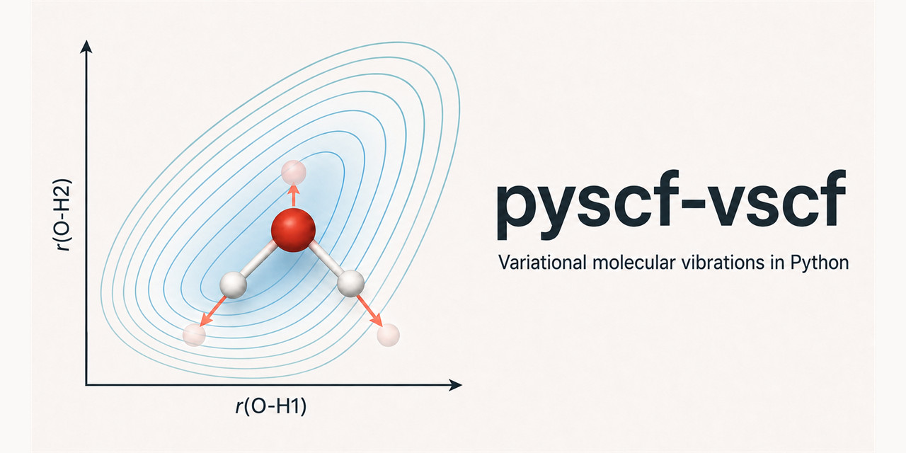
pyscf-vscf computes anharmonic vibrational spectra variationally, on
potential-energy and dipole-moment surfaces evaluated with
PySCF. It scans one or two bond stretches (or a normal
coordinate), solves the vibrational Schrodinger equation on that grid, and
reports assigned transition frequencies with absolute infrared intensities.
For more coordinates it offers vibrational self-consistent field (VSCF) and
configuration-interaction (VCI) solvers on fitted n-mode surfaces.
It is meant for researchers who need anharmonic frequencies and intensities of a few strongly anharmonic modes, such as X-H stretches, overtones, and isotopologues, beyond what harmonic analysis or second-order perturbation theory provide, and who want every step to be inspectable, cached, and reproducible from Python.
Install
pip install pyscf-vscf
Python 3.11 or newer. PySCF and geomeTRIC are installed with the package. PySCF does not support native Windows, so Windows users should install under WSL. See the installation guide for development installs, parallelism, and memory. Upgrading from 0.2? See the migration guide.
Quickstart
Optimize a geometry, then compute the O-H stretch spectrum of water from a potential and dipole scan around the optimized bond length:
pyscf-vscf opt water.xyz --method b3lyp --basis cc-pvdz
pyscf-vscf scan1d water-opt.xyz --bond 0-1 --method b3lyp --basis cc-pvdz \
    --store water.sqlite --output oh.npz
v  nu/cm^-1   mu_axis/D   I_axis/(km/mol)   int_axis/(m^2/s)   orientation: polarized along bond axis
1   3644.8     2.6930e-02     1.9877e+01     6.2173e-11
2   7136.8    -8.8835e-03     4.2353e+00     1.3247e-11
3  10481.2     2.0528e-03     3.3214e-01     1.0389e-12
4  13683.0    -4.9706e-04     2.5422e-02     7.9517e-14
Bonds are zero-based atom indices. The 41 points run in parallel
automatically; this scan takes about 11 s on an 8-core machine. --store keeps every
electronic point in a SQLite file, so an interrupted or partly failed scan
resumes where it stopped. --output writes the finished scan, from which
spectra are recomputed without electronic-structure calculations, for any
isotopologue on the same surface (the file supplies the method):
pyscf-vscf scan1d water-opt.xyz --bond 0-1 --reuse oh.npz --states 6 --intensity both
Check that the grid is wide and dense enough for the states you report.
Without --range MIN MAX NPTS, the grid runs from 0.40 A inside to 0.70 A
outside the bond length in the input geometry, with 41 points: a starting
point chosen by benchmark on O-H, H-Cl, C-O, and C-C bonds
(scans). States that place more than 1e-5 of their
probability on the outermost grid points are marked with * and need a
wider range. The mark does not detect a grid that is too coarse, so also
confirm that the reported states do not change when you add points.
Other commands: pyscf-vscf harmonic (harmonic frequencies), scan2d (two
coupled bond stretches), scan1d --coordinate normal|normal-relaxed, and
inspect FILE (describe a scan file or point store). Run
pyscf-vscf COMMAND --help for every option; --json results.json also
writes machine-readable results.
Python
The same workflow from Python: plan the scan, run it (optionally in parallel and resumably), and solve the vibrational problem:
from pyscf_vscf import (
    ESSettings, PointStore, PySCFMeanFieldProvider, RunnerSettings,
    bond_spectrum, plan_bond_scan, read_geometry, run_scan,
)

def main():
    water = read_geometry("water-opt.xyz")
    provider = PySCFMeanFieldProvider(ESSettings(method="b3lyp", basis="cc-pvdz"))
    plan = plan_bond_scan(water, provider, ["0-1"])          # default grid
    with PointStore("water.sqlite") as store:
        scan = run_scan(plan, provider, store=store, settings=RunnerSettings(workers=4))
    for record in bond_spectrum(scan, water, max_state_index=3):
        print(record.quanta, round(record.frequency_cm, 1))


if __name__ == "__main__":    # workers are spawned processes that import this file
    main()
Any PySCF method can be used through a MethodRecipe: a module-level
function that configures the mean field, plus a manifest that identifies it.
Recipes work in scans, n-mode plans, harmonic analysis, and optimization, and
on the command line with --recipe MODULE:NAME:
from pyscf_vscf import MethodRecipe, PySCFMeanFieldProvider

def wb97mv(mol):
    mf = mol.RKS(xc="wb97m-v").density_fit()
    mf.grids.level = 4
    return mf                                            # configured, not run

recipe = MethodRecipe(
    recipe_id="mylab.wb97m-v", recipe_version="1", basis="def2-tzvp",
    configuration={"xc": "wb97m-v", "grids_level": 4, "density_fit": "default"},
    mean_field=wb97mv,
)
provider = PySCFMeanFieldProvider(factory=recipe)
VSCF and VCI on n-mode surfaces need no electronic-structure code of their own; this model runs in a second:
import numpy as np
from pyscf_vscf import NModePotential, vscf_spectrum

q1 = np.linspace(-0.35, 0.35, 31)
q2 = np.linspace(-0.30, 0.30, 29)
model = NModePotential(
    coordinates=(q1, q2),                       # angstrom
    masses_amu=(1.0, 1.5),
    one_mode_potentials_Eh=(0.08 * q1**2, 0.11 * q2**2),
    two_mode_couplings_Eh={(0, 1): 0.20 * q1[:, None] ** 2 * q2[None, :] ** 2},
)
spectrum = vscf_spectrum(model, max_quanta_per_mode=2, max_total_quanta=2)
for transition in spectrum.transitions:
    print(transition.quanta, round(transition.frequency_cm, 1))
python -m pyscf_vscf.examples.water_vscf_vci runs the whole chain for water:
optimization, harmonic modes, a 1MR/2MR n-mode surface from PySCF points,
then VSCF and VCI fundamentals with intensities. vscf_two_mode and
nmode_vci are smaller examples without electronic-structure calculations.
What it computes
- 1D and 2D sinc-DVR spectra on frozen local-bond scans, rigid normal-coordinate scans, and exactly constrained relaxed normal-coordinate scans, with overlap-based state assignments.
- Absolute intensities for light polarized along a bond and for isotropic samples, in km/mol and as integrated cross sections.
- State-specific VSCF for n-mode Hamiltonians with one-mode potentials and two-mode couplings, with transition moments and intensities.
- Fitted 1MR/2MR and selected 3MR scalar and vector n-mode surfaces, VCI on
VSCF modals, and a complete triatomic Jacobi
J=0kinetic-energy operator. - Harmonic analysis and geometry optimization through PySCF and geomeTRIC, with the built-in methods or any PySCF method as a recipe.
- Resumable, parallel evaluation of electronic points with a SQLite point store, and checksummed scan files whose identity is independent of isotope masses.
The package does not generate full-dimensional potential surfaces and does not implement a general curvilinear or rovibrational kinetic-energy operator. Reduced-dimensional results inherit the error of the omitted coordinates.
Stability
| Area | Modules | Status |
|---|---|---|
| Command line, scans, point store and runner, 1D/2D DVR spectra, method recipes | cli, scans, runner, point_store, contracts, variational, dvr, backends.pyscf |
Stable; changes are announced in the changelog |
| VSCF on n-mode potentials | vscf |
Stable |
n-mode surfaces, triatomic J=0, VCI, transition moments, multilevel surfaces, correlated providers |
nmode, kinetic, vci, transition_moments, multilevel, backends.pyscf_correlated |
Evolving; may change between minor releases |
0.4 removed the APIs deprecated in 0.3 (the 0.2 tuple scans, schema-3 cache writers and loaders, and the flag-style command line); 0.2 caches remain readable. See the migration guide.
Documentation
The documentation site has
tutorials, guides, and the API reference. The guides are also in docs/:
- Scans, the point store, and parallel runs
- Migrating from 0.2
- Reusing points and scans
- Intensity conventions
- Advanced n-mode and VCI guide
- Correlated and finite-field providers
- Running the validations
- Changelog and roadmap
Validation
The test suite combines analytic numerical checks, small PySCF calculations, and archived H2O/HDO/D2O and NH3 molecular validations against exact DVR. These establish solver correctness and convergence on the stated reduced-dimensional Hamiltonians; they do not establish general spectroscopic accuracy.
Citing and contributing
If you use pyscf-vscf in research, cite it with the metadata in
CITATION.cff
(GitHub's "Cite this repository" button). Bug reports, questions, and
contributions are welcome; see
CONTRIBUTING.
License
The code is MIT-licensed. The archived validation data are licensed under
CC BY 4.0; see
DATA_LICENSE.md.
1 maintainer

Metadata
1 maintainer
Release files for pyscf-vscf 0.4.0
For a detailed explanation of source distributions (sdists) and built distributions (wheels), please see the package formats documentation.
Source distribution (sdist)
| File | Size | Uploaded | |
|---|---|---|---|
| pyscf_vscf-0.4.0.tar.gz | 1.2 MB | Details |
Built distribution (wheel)
| File | Interpreter | ABI | Platform | Reset |
|---|---|---|---|---|
| pyscf_vscf-0.4.0-py3-none-any.whl | Python 3 | none | any | Details |
Total release size: 1.4 MB
Release files / pyscf_vscf-0.4.0.tar.gz
| Download URL | pyscf_vscf-0.4.0.tar.gz |
|---|---|
| Size | 1.2 MB |
| Tags | Source |
|
SHA-256 checksum How to use checksums |
866ad1358b991be153f28b58fcef9516fa3baf05a6f3d759d438891c3074c334
|
|
BLAKE2b-256 checksum How to use checksums |
ff914ff21e890ab0186e93c1f8ff78908f75d44ae5bd05cb5a1da890b017f799
|
| Upload date | |
|
Uploaded using Trusted Publishing? What is trusted publishing? |
Yes |
| Uploaded via |
twine/7.0.0 CPython/3.13.14
|
Provenance
Provenance describes where a file came from. On PyPI, provenance is shared via attestations, which provide a verifiable record of the build or publishing details. View details, limitations and caveats.


PyPI Publish Attestation
PyPI verified that this artifact, at this checksum, originated from the publisher listed below.
Signed by GitHub Actions, verified by PyPI on Oct 12, 2026.
Transparency logRelease files / pyscf_vscf-0.4.0-py3-none-any.whl
| Download URL | pyscf_vscf-0.4.0-py3-none-any.whl |
|---|---|
| Size | 211.0 kB |
| Tags | Python 3 |
|
SHA-256 checksum How to use checksums |
b043aac6eb293bafbd19a05cbea7f64fc2758834015e34ac6f5db2a5e81990e4
|
|
BLAKE2b-256 checksum How to use checksums |
f66b5bd9190e2b8ef992316d011d33304f24f6f9c1425d0dd7a13aafa2f0fe30
|
| Upload date | |
|
Uploaded using Trusted Publishing? What is trusted publishing? |
Yes |
| Uploaded via |
twine/7.0.0 CPython/3.13.14
|
Provenance
Provenance describes where a file came from. On PyPI, provenance is shared via attestations, which provide a verifiable record of the build or publishing details. View details, limitations and caveats.
PyPI Publish Attestation
PyPI verified that this artifact, at this checksum, originated from the publisher listed below.
Signed by GitHub Actions, verified by PyPI on Oct 12, 2026.
Transparency log













