
rangedf
Transform Tick Data into OHLCV Range Dataframe!
Installation
pip install rangedf
or just copy rangedf.py file to your project!
- rangedf requires pandas, numpy and mplfinance
Content
Usage
There are two classes available:
Range(df, range_size)
To create Range OHLCV dataframe with existing Ticks data.RangeWS(timestamp, price, range_size, external_df, ts_unit)
To create real-time Range charts, usually over a WebSocket connection.
Let's start with the first class, load a Pandas DataFrame containing Ticks Data, for example:
import pandas as pd
df_ticks = pd.read_parquet('examples/data/EURGBP_T1_cT.parquet')
df_ticks.rename(columns={'bid': 'close'}, inplace=True)
df_ticks.head(5)
| ask | close | spread | |
|---|---|---|---|
| datetime | |||
| 2025-05-08 00:00:00.678 | 0.85047 | 0.85043 | 0.00004 |
| 2025-05-08 00:00:00.848 | 0.85047 | 0.85045 | 0.00002 |
| 2025-05-08 00:00:02.000 | 0.85046 | 0.85045 | 0.00001 |
| 2025-05-08 00:00:02.246 | 0.85048 | 0.85046 | 0.00002 |
| 2025-05-08 00:00:02.447 | 0.85048 | 0.85045 | 0.00003 |
Only two columns are required:
close: Mandatory.datetime: If is not present, the index will be used.
After importing rangedf and setting range_size, just call range_df() with the choosen mode.
See all available modes in rangedf_modes.ipynb
from rangedf import Range
r = Range(df_ticks, range_size=0.0003)
df = r.range_df(utils_columns=False) # utils-columns => [direction, tick_index_open, tick_index_close]
df.head(5)
| open | high | low | close | volume | |
|---|---|---|---|---|---|
| datetime | |||||
| 2025-05-08 00:20:02.244 | 0.85052 | 0.85077 | 0.85047 | 0.85077 | 560 |
| 2025-05-08 00:37:55.846 | 0.85077 | 0.85103 | 0.85073 | 0.85103 | 358 |
| 2025-05-08 00:55:00.448 | 0.85105 | 0.85112 | 0.85082 | 0.85082 | 532 |
| 2025-05-08 00:57:40.643 | 0.85081 | 0.85096 | 0.85066 | 0.85066 | 246 |
| 2025-05-08 01:08:23.446 | 0.85066 | 0.85079 | 0.85049 | 0.85049 | 716 |
You can use mpf.plot() or r.plot(), as in the example below.
import mplfinance as mpf
mpf.plot(df.iloc[:130], type='candle', volume=True, style="charles",
         title=f"Range: normal\nrange_size: 0.0003")
mpf.show()
# same as:
# r.plot('normal')

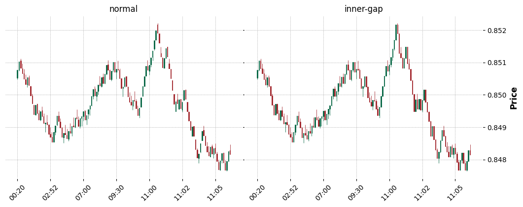
As described in rangedf_modes.ipynb, we can have multiple dataframes of different modes from the same instance.
df_normal = r.range_df()
df_nongap = r.range_df('inner-gap')

fig = mpf.figure(style='charles', figsize=(12.5,9))
fig.subplots_adjust(hspace=0.1, wspace=0.01)
ax1 = fig.add_subplot(2,2,1)
ax2 = fig.add_subplot(2,2,2)

mpf.plot(df_normal.iloc[:130],type='candle',ax=ax1,axtitle='normal')
mpf.plot(df_nongap.iloc[:130],type='candle',ax=ax2,axtitle='inner-gap')
mpf.show()
Animation/Real-time Range Chart
To run the animation examples, clone this repository, then into the rangedf/examples folder, run:,
- python ws_animchart_demo.py,
- python ws_multichart_demo.py,
- python ws_externaldf_demo.py
NOTE: There are comments, in each of above example files, talking about situations or recommendations to be applied in real cases.
Performance-wise
From v2.0, the Range calculation is powered by numpy arrays instead of python dicts/list as before, the OHLC variations (modes) are also calculated all at once, leading to a massive speed-up in Range Charts creation.
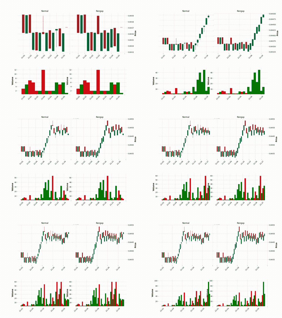
Regarding "backtest vs real-time" charts, there are 2 tests about the OHLCV reliability between them.
The tests includes creating charts from scratch or using external data (Range.to_rws())
Is the Range chart calculated correctly?
I asked myself the same question, how about we see for ourselves?
We are going to do this based on Spotware's FX/CFD Trading Platform called cTrader,
using IC Markets/Trading as Price Provider.
Let's go!
RESUME: Despite the possible occurrence of more/less bars in cases of gap, the range calculation is practically the same or very approximate.
Non-Affiliation Disclaimer
I'm not endorsed by, directly affiliated with, maintained, authorized, or sponsored by any company previously mentioned. All product and company names are the registered trademarks of their original owners. The use of any trade name or trademark is for identification and reference purposes only and does not imply any association with the trademark holder of their product brand.
1 maintainer

Metadata
1 maintainer
Release files for rangedf 2.1
For a detailed explanation of source distributions (sdists) and built distributions (wheels), please see the package formats documentation.
Source distribution (sdist)
| File | Size | Uploaded | |
|---|---|---|---|
| rangedf-2.1.tar.gz | 14.2 kB | Details |
Built distribution (wheel)
| File | Interpreter | ABI | Platform | Reset |
|---|---|---|---|---|
| rangedf-2.1-py3-none-any.whl | Python 3 | none | any | Details |
Total release size: 24.6 kB
Release files / rangedf-2.1.tar.gz
| Download URL | rangedf-2.1.tar.gz |
|---|---|
| Size | 14.2 kB |
| Tags | Source |
|
SHA-256 checksum How to use checksums |
fd6800ddfbaa38f900a6ae6de78d75b0f26926723c602472c38dd2adb3d1fea9
|
|
BLAKE2b-256 checksum How to use checksums |
0d67220e2956c0b261433cc3a35346fc9d3c01e53de677e3b4dec9e85df2927f
|
| Upload date | |
|
Uploaded using Trusted Publishing? What is trusted publishing? |
No |
| Uploaded via |
twine/7.0.0 CPython/3.14.7
|
Release files / rangedf-2.1-py3-none-any.whl
| Download URL | rangedf-2.1-py3-none-any.whl |
|---|---|
| Size | 10.4 kB |
| Tags | Python 3 |
|
SHA-256 checksum How to use checksums |
f9de73868e1fc94fcf7babeb899b3c7d7b79b7776aa8929ff9dd30e9c71d318b
|
|
BLAKE2b-256 checksum How to use checksums |
b31502d6f610da230772cf39dab461fd0f1d61c9892ade5868421bd6ded042f3
|
| Upload date | |
|
Uploaded using Trusted Publishing? What is trusted publishing? |
No |
| Uploaded via |
twine/7.0.0 CPython/3.14.7
|














