RiskOptima is a powerful Python toolkit for financial risk analysis, portfolio optimization, and advanced quantitative modeling. It integrates state-of-the-art methodologies, including Monte Carlo simulations, Value at Risk (VaR), Conditional VaR (CVaR), Black-Scholes, Heston, and Merton Jump Diffusion models, to aid investors in making data-driven investment decisions.

Project description
RiskOptima


RiskOptima is a comprehensive Python toolkit for evaluating, managing, and optimizing investment portfolios. This package is designed to empower investors and data scientists by combining financial risk analysis, backtesting, mean-variance optimization, and machine learning capabilities into a single, cohesive package.
Stats
https://pypistats.org/packages/riskoptima
Key Features
- Modular Core:
MarketData,Portfolio, andBacktestConfigtypes for clean workflows. - Backtesting Framework: Strategy interfaces, cost/slippage modeling, and performance tracking.
- Risk Models: Factor risk model with exposures and factor-based covariance estimation.
- Optimization: Mean-variance, efficient frontier, max Sharpe, and constraint handling (bounds, leverage, turnover, factor limits).
- Risk Management: VaR, CVaR, volatility, and drawdown analytics.
- Monte Carlo Simulations: Analyze potential portfolio outcomes. See example here https://github.com/JordiCorbilla/efficient-frontier-monte-carlo-portfolio-optimization
- Market & Allocation Visuals: Correlation matrices, portfolio area charts, and diagnostics.
- Quant Models: Black-Litterman, stochastic volatility models, and options/Greeks analytics.
- Portfolio Projects: algorithmic trading/backtesting, portfolio optimization, market risk dashboard, option pricing engine, and credit risk model workflows.
Quant Portfolio Project Map
| Project | Notebook / Example | Package API | Screenshot |
|---|---|---|---|
| Algorithmic Trading Backtester | 05-portfolio_sma_strategy.ipynb |
riskoptima.backtest |
 |
| Portfolio Optimization | 02-portfolio_optimization_riskoptima.ipynb |
riskoptima.optim |
 |
| Market Risk Dashboard | examples/example_market_risk_dashboard.py |
riskoptima.reporting |
 |
| Option Pricing Engine | examples/example_option_pricing_engine.py |
riskoptima.options |
 |
| Credit Risk Model | 08-credit_risk_model_demo.ipynb |
riskoptima.credit |
 |
See docs/quant_project_map.md for a recruiter/interviewer-friendly walkthrough of the five projects.
Installation
See the project here: https://pypi.org/project/riskoptima/
pip install riskoptima
Usage
New modular API (backtest + factor risk + constraints)
import pandas as pd
from riskoptima import FactorRiskModel, Constraints, optimize_max_sharpe
from riskoptima import SMACrossStrategy, run_backtest, BacktestConfig, SimpleCostModel

# prices: DataFrame with Date index and asset columns
prices = pd.read_csv("prices.csv", index_col=0, parse_dates=True)
asset_returns = prices.pct_change().dropna()

# factors: Fama-French returns DataFrame (e.g. from RiskOptima.get_fff_returns)
factors = pd.read_csv("fama_french_factors.csv", index_col=0, parse_dates=True)

factor_model = FactorRiskModel(factor_returns=factors).fit(asset_returns)
factor_cov = factor_model.covariance_matrix()

constraints = Constraints(factor_bounds={"MKT": (-0.2, 0.8)})
weights = optimize_max_sharpe(
    expected_returns=asset_returns.mean() * 252,
    cov=factor_cov,
    constraints=constraints,
    factor_exposures=factor_model.exposures,
    risk_free_rate=0.02,
)

strategy = SMACrossStrategy(short_window=20, long_window=50)
config = BacktestConfig(initial_cash=1_000_000, rebalance_rule="D")
cost_model = SimpleCostModel(spread_bps=2.0, impact_coeff=0.0)
equity_curve, weights_history = run_backtest(prices, strategy, config, cost_model)
See examples/example_factor_backtest.py for a runnable end-to-end example.
Offline sample datasets
RiskOptima includes small synthetic datasets for deterministic examples:
data/synthetic_market_returns.csvdata/synthetic_credit_portfolio.csv
These are intentionally small and have no external data dependency.
Credit Risk Model
RiskOptima includes a production-ready credit risk layer for PD/LGD/EAD portfolios, expected loss, unexpected loss, rating migration, Merton structural default probability, and Credit VaR/CVaR Monte Carlo.
import pandas as pd
from riskoptima.credit import (
    expected_loss,
    portfolio_expected_loss,
    simulate_credit_losses,
    credit_var,
    credit_cvar,
    merton_pd,
)

portfolio = pd.DataFrame({
    "obligor": ["A", "B", "C"],
    "PD": [0.01, 0.025, 0.04],
    "LGD": [0.40, 0.45, 0.55],
    "EAD": [1_000_000, 750_000, 500_000],
})

print(expected_loss(0.02, 0.45, 1_000_000))
print(portfolio_expected_loss(portfolio))

losses = simulate_credit_losses(portfolio, n_sims=20_000, random_state=42)
print(credit_var(losses, confidence=0.99))
print(credit_cvar(losses, confidence=0.99))
print(merton_pd(asset_value=150, debt_face_value=100, asset_vol=0.25, risk_free_rate=0.03, maturity=1.0))
See 08-credit_risk_model_demo.ipynb for an end-to-end notebook.
Market Risk Dashboard
RiskOptima can build a dashboard-ready market risk report with annualized return, volatility, Sharpe, Sortino, drawdown, historical VaR, Gaussian VaR, CVaR/expected shortfall, beta, tracking error, information ratio, rolling volatility, and rolling drawdown.
Screenshot placeholder: plots/market_risk_dashboard.png
import pandas as pd
from riskoptima.reporting import build_market_risk_report

returns = pd.DataFrame({
    "AssetA": [0.01, -0.005, 0.004, 0.002],
    "AssetB": [0.002, 0.003, -0.006, 0.005],
})
weights = pd.Series({"AssetA": 0.6, "AssetB": 0.4})

report = build_market_risk_report(returns, weights=weights, confidence_levels=(0.95, 0.99))
print(report.metrics["annualized_volatility"])
print(report.metrics["historical_var"][0.99])
Run examples/example_market_risk_dashboard.py to generate a multi-panel dashboard.
Optional Streamlit dashboard:
pip install streamlit
streamlit run examples/streamlit_market_risk_dashboard.py
Option Pricing Engine
The clean options API covers Black-Scholes call/put pricing, Greeks, implied volatility, binomial trees, and Monte Carlo European option pricing while preserving the legacy RiskOptima class methods.
import pandas as pd
from riskoptima.options import (
    black_scholes_price,
    black_scholes_greeks,
    implied_volatility,
    monte_carlo_european_option,
)

S, K, T, r, sigma = 100, 100, 1.0, 0.05, 0.20
call = black_scholes_price(S, K, T, r, sigma, option_type="call")
put = black_scholes_price(S, K, T, r, sigma, option_type="put")
greeks = pd.Series(black_scholes_greeks(S, K, T, r, sigma, option_type="call"))
iv = implied_volatility(call, S, K, T, r, option_type="call")
mc = monte_carlo_european_option(S, K, T, r, sigma, option_type="call", random_state=42)

print(call, put)
print(greeks)
print(iv, mc)
Run examples/example_option_pricing_engine.py for a full pricing comparison.
Example 1: Setting up your portfolio
Create your portfolio table similar to the below:
| Asset | Weight | Label | MarketCap |
|---|---|---|---|
| MO | 0.04 | Altria Group Inc. | 110.0e9 |
| NWN | 0.14 | Northwest Natural Gas | 1.8e9 |
| BKH | 0.01 | Black Hills Corp. | 4.5e9 |
| ED | 0.01 | Con Edison | 30.0e9 |
| PEP | 0.09 | PepsiCo Inc. | 255.0e9 |
| NFG | 0.16 | National Fuel Gas | 5.6e9 |
| KO | 0.06 | Coca-Cola Company | 275.0e9 |
| FRT | 0.28 | Federal Realty Inv. Trust | 9.8e9 |
| GPC | 0.16 | Genuine Parts Co. | 25.3e9 |
| MSEX | 0.05 | Middlesex Water Co. | 2.4e9 |
import pandas as pd
from riskoptima import RiskOptima

import warnings
warnings.filterwarnings(
    "ignore",
    category=FutureWarning,
    message=".*DataFrame.std with axis=None is deprecated.*"
)

# Define your current porfolio with your weights and company names
asset_data = [
    {"Asset": "MO",    "Weight": 0.04, "Label": "Altria Group Inc.",       "MarketCap": 110.0e9},
    {"Asset": "NWN",   "Weight": 0.14, "Label": "Northwest Natural Gas",   "MarketCap": 1.8e9},
    {"Asset": "BKH",   "Weight": 0.01, "Label": "Black Hills Corp.",         "MarketCap": 4.5e9},
    {"Asset": "ED",    "Weight": 0.01, "Label": "Con Edison",                "MarketCap": 30.0e9},
    {"Asset": "PEP",   "Weight": 0.09, "Label": "PepsiCo Inc.",              "MarketCap": 255.0e9},
    {"Asset": "NFG",   "Weight": 0.16, "Label": "National Fuel Gas",         "MarketCap": 5.6e9},
    {"Asset": "KO",    "Weight": 0.06, "Label": "Coca-Cola Company",         "MarketCap": 275.0e9},
    {"Asset": "FRT",   "Weight": 0.28, "Label": "Federal Realty Inv. Trust", "MarketCap": 9.8e9},
    {"Asset": "GPC",   "Weight": 0.16, "Label": "Genuine Parts Co.",         "MarketCap": 25.3e9},
    {"Asset": "MSEX",  "Weight": 0.05, "Label": "Middlesex Water Co.",       "MarketCap": 2.4e9}
]
asset_table = pd.DataFrame(asset_data)

capital = 100_000

asset_table['Portfolio'] = asset_table['Weight'] * capital

ANALYSIS_START_DATE = RiskOptima.get_previous_year_date(RiskOptima.get_previous_working_day(), 1)
ANALYSIS_END_DATE   = RiskOptima.get_previous_working_day()
BENCHMARK_INDEX     = 'SPY'
RISK_FREE_RATE      = 0.05
NUMBER_OF_WEIGHTS   = 10_000
NUMBER_OF_MC_RUNS   = 1_000
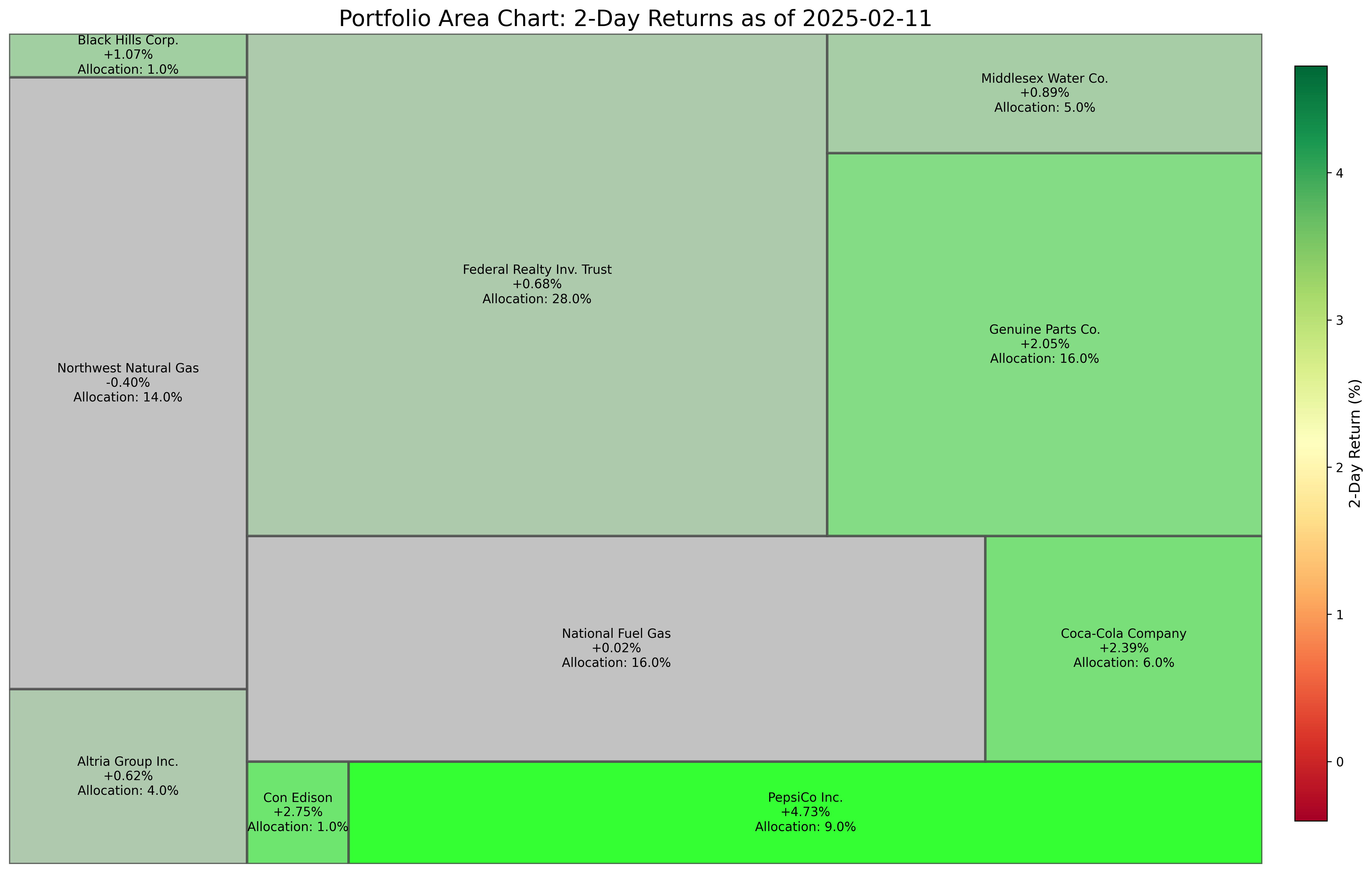
Example 1: Creating a Portfolio Area Chart
If you want to know visually how's your portfolio doing right now
RiskOptima.create_portfolio_area_chart(
    asset_table,
    end_date=ANALYSIS_END_DATE,
    lookback_days=2,
    title="Portfolio Area Chart"
)
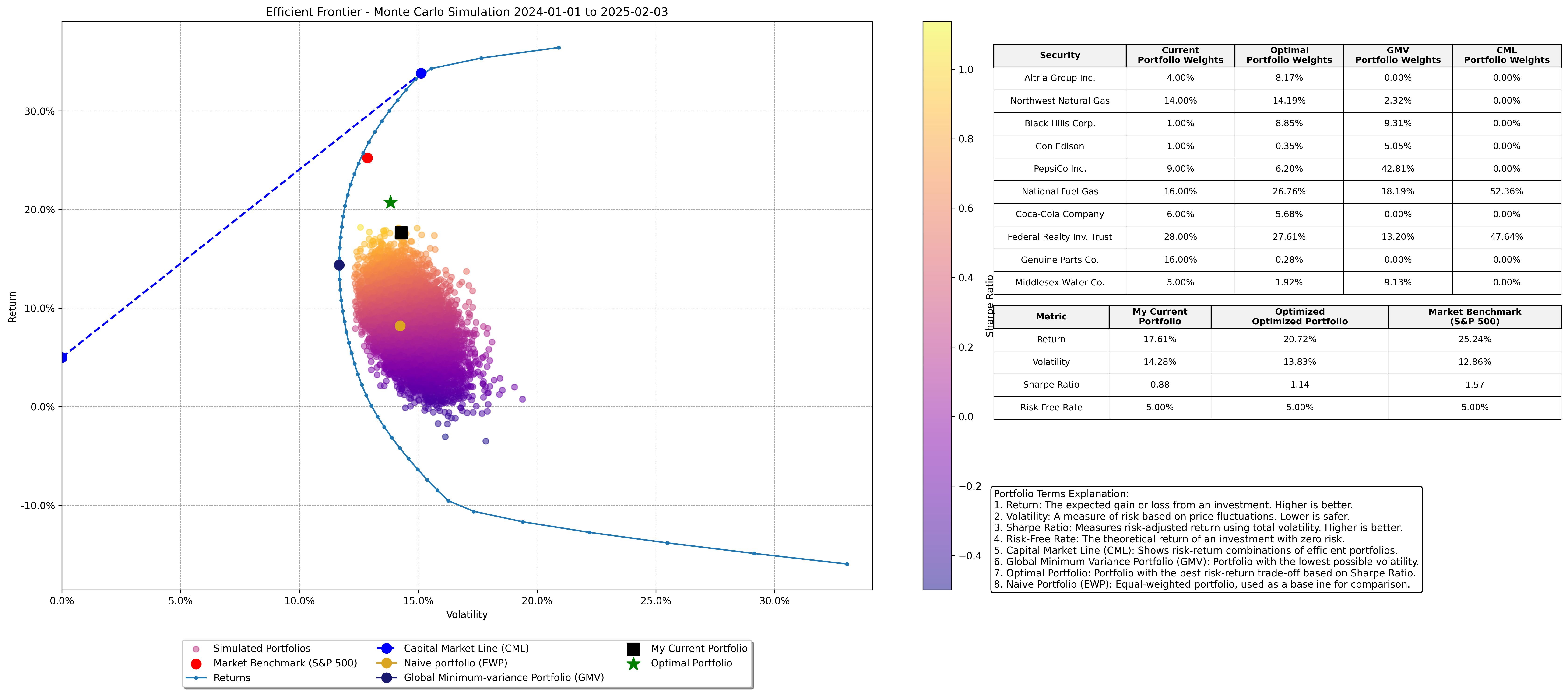
Example 2: Efficient Frontier - Monte Carlo Portfolio Optimization
RiskOptima.plot_efficient_frontier_monte_carlo(
    asset_table,
    start_date=ANALYSIS_START_DATE,
    end_date=ANALYSIS_END_DATE,
    risk_free_rate=RISK_FREE_RATE,
    num_portfolios=NUMBER_OF_WEIGHTS,
    market_benchmark=BENCHMARK_INDEX,
    set_ticks=False,
    x_pos_table=1.15,    # Position for the weight table on the plot
    y_pos_table=0.52,    # Position for the weight table on the plot
    title=f'Efficient Frontier - Monte Carlo Simulation {ANALYSIS_START_DATE} to {ANALYSIS_END_DATE}'
)
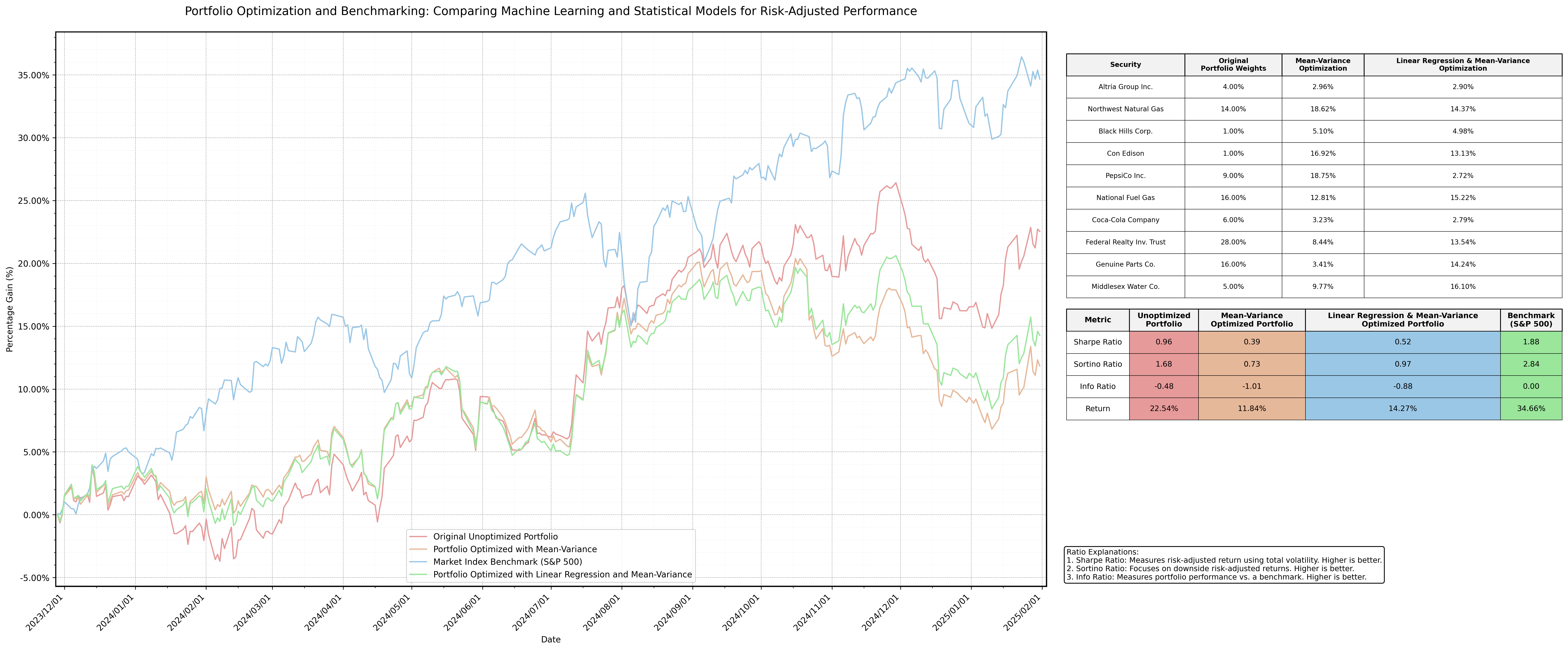
Example 3: Portfolio Optimization using Mean Variance and Machine Learning
RiskOptima.run_portfolio_optimization_mv_ml(
    asset_table=asset_table,
    training_start_date='2022-01-01',
    training_end_date='2023-11-27',
    model_type='Linear Regression',
    risk_free_rate=RISK_FREE_RATE,
    num_portfolios=100000,
    market_benchmark=[BENCHMARK_INDEX],
    max_volatility=0.25,
    min_weight=0.03,
    max_weight=0.2
)
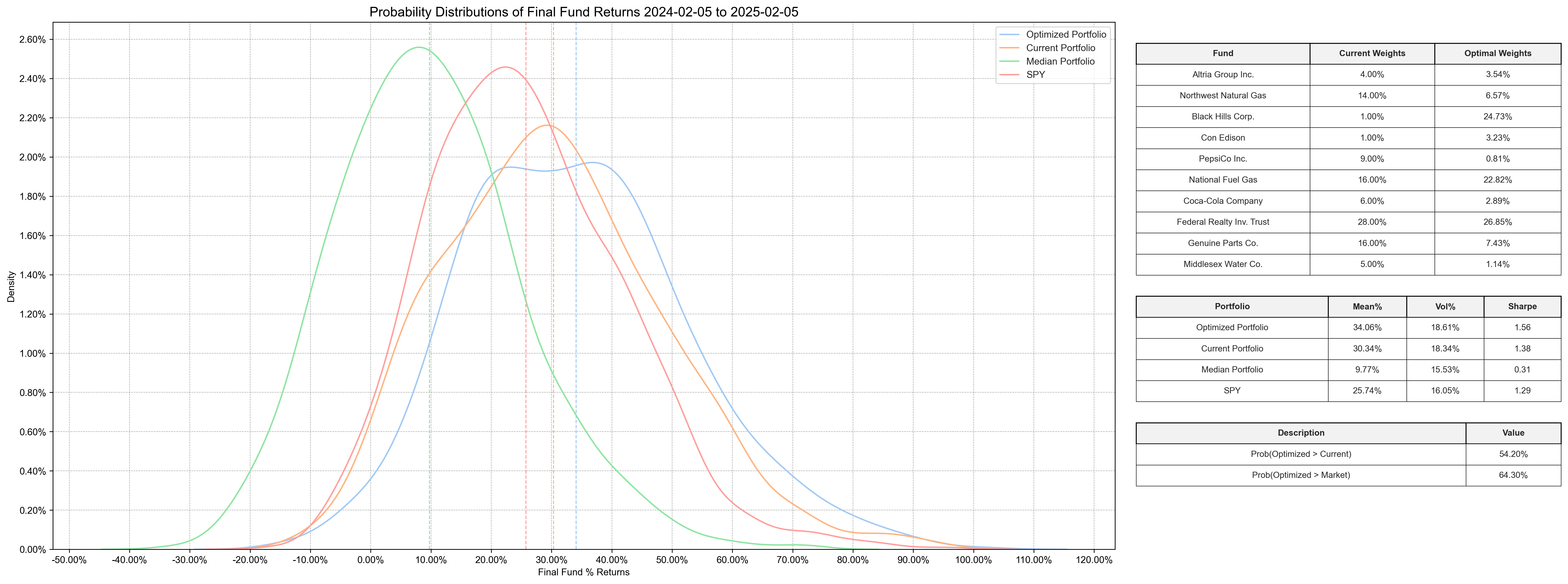
Example 4: Portfolio Optimization using Probability Analysis
RiskOptima.run_portfolio_probability_analysis(
    asset_table=asset_table,
    analysis_start_date=ANALYSIS_START_DATE,
    analysis_end_date=ANALYSIS_END_DATE,
    benchmark_index=BENCHMARK_INDEX,
    risk_free_rate=RISK_FREE_RATE,
    number_of_portfolio_weights=NUMBER_OF_WEIGHTS,
    trading_days_per_year=RiskOptima.get_trading_days(),
    number_of_monte_carlo_runs=NUMBER_OF_MC_RUNS
)
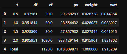
Example 5: Macaulay Duration
from riskoptima import RiskOptima
cf = RiskOptima.bond_cash_flows_v2(4, 1000, 0.06, 2)  # 2 years, semi-annual, hence 4 periods
md_2 = RiskOptima.macaulay_duration_v3(cf, 0.05, 2)
md_2
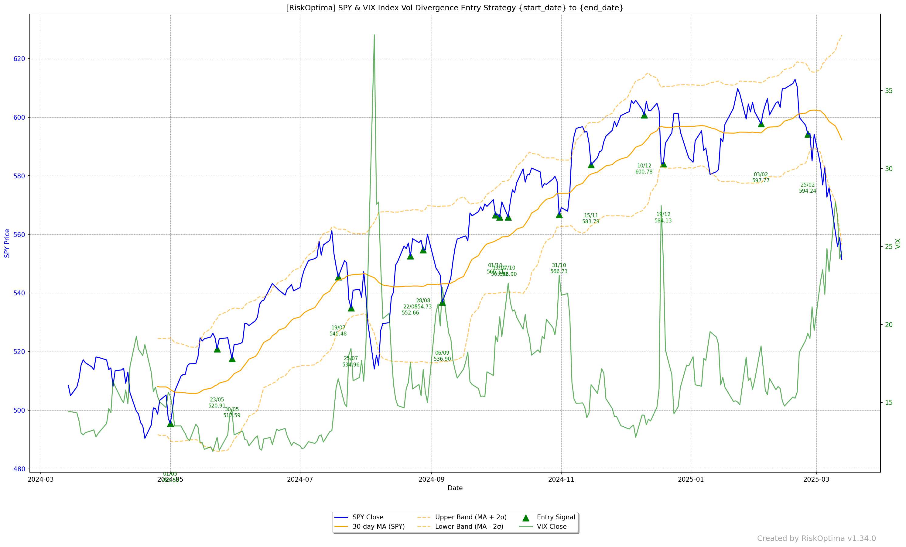
Example 6: Market Turns with SPY & VIX Divergence
ANALYSIS_START_DATE = RiskOptima.get_previous_year_date(RiskOptima.get_previous_working_day(), 1)
ANALYSIS_END_DATE   = RiskOptima.get_previous_working_day()

df_signals, df_exits, returns = RiskOptima.run_index_vol_divergence_signals(start_date=ANALYSIS_START_DATE,
                                                                            end_date=ANALYSIS_END_DATE)
Documentation
For complete documentation and usage examples, visit the GitHub repository:
Contributing
We welcome contributions! If you'd like to improve the package or report issues, please visit the GitHub repository.
License
RiskOptima is licensed under the MIT License.
Support me
Release history Release notifications | RSS feed


Download files
Download the file for your platform. If you're not sure which to choose, learn more about installing packages.
Source Distribution
Built Distribution
Filter files by name, interpreter, ABI, and platform.
If you're not sure about the file name format, learn more about wheel file names.
Copy a direct link to the current filters
File details
Details for the file riskoptima-2.3.0.tar.gz.
File metadata
- Download URL: riskoptima-2.3.0.tar.gz
- Upload date:
- Size: 59.6 kB
- Tags: Source
- Uploaded using Trusted Publishing? No
- Uploaded via: poetry/1.8.5 CPython/3.12.7 Windows/11
File hashes
| Algorithm | Hash digest | |
|---|---|---|
| SHA256 |
89cdbd0710682c1f2c6ab4185b5e71ef907e3a97e4854c1f63a28e3a1402623b
|
|
| MD5 |
fb771df436e56b1f4f5e2d8524fd6a7a
|
|
| BLAKE2b-256 |
fda660f523c4fbed7d9cb6e93a3454130a381f5ce506bfc7ee89f74ea39beae3
|
File details
Details for the file riskoptima-2.3.0-py3-none-any.whl.
File metadata
- Download URL: riskoptima-2.3.0-py3-none-any.whl
- Upload date:
- Size: 64.7 kB
- Tags: Python 3
- Uploaded using Trusted Publishing? No
- Uploaded via: poetry/1.8.5 CPython/3.12.7 Windows/11
File hashes
| Algorithm | Hash digest | |
|---|---|---|
| SHA256 |
1b85cacb29677945462989ff0ac9c1b18946bdaf62ba3f2e192c652d28c46886
|
|
| MD5 |
5c489d444a3c214e2286da3c0322bcd8
|
|
| BLAKE2b-256 |
264f56fd55470bea045c91fa46cfebb1d4ef044751a15b54829cab2fff230c29
|


