
scope-profiler
Profile Python code regions—and optionally C, Fortran, MPI, NVTX, and LIKWID—with one consistent API and HDF5 output format.
pip install scope-profiler
Quick start
from scope_profiler import ProfileManager

with ProfileManager.session():
    @ProfileManager.profile("main")
    def main():
        with ProfileManager.profile_region("work"):
            sum(range(100))  # replace with the code you want to measure

    main()
# writes profiling_data.h5 and prints a summary
Create independent managers when two profiling sessions need to coexist. Each manager records only calls made through that manager and writes its own output:
compute_profiler = ProfileManager()
io_profiler = ProfileManager()

with compute_profiler.session(file_path="compute.h5", verbose=False):
    with io_profiler.session(file_path="io.h5", verbose=False):
        with compute_profiler.profile_region("solve"):
            solve()
        with io_profiler.profile_region("checkpoint"):
            write_checkpoint()
These are independent nested sessions. LIKWID’s marker state is
process-global, so only one overlapping session may use
use_likwid=True.
Concurrency is a separate switch. track_threads=True gives every
thread its own buffers and its own lane in the reconstructed call graph,
and reports each thread’s name, lifetime and CPU time;
track_async=True does the same for asyncio tasks and greenlets, and
splits every call into the time its task held the thread and the time it
spent awaiting:
with ProfileManager.session(track_async=True, return_results=True) as run:
    asyncio.run(main())

fetch = run.results["fetch"][0]
fetch.durations - fetch.await_times     # time actually spent running
for task in run.results.tasks[0]:
    print(task.name, task.running_time, task.awaiting_time)
You can also profile a script without changing its source:
scope-profiler run my_script.py
scope-profiler inspect profiling_data.h5
scope-profiler plot default profiling_data.h5 -o figures
scope-profiler report profiling_data.h5 -o report.html
Profile a pytest suite
The installed package provides an opt-in pytest plugin. It records one region for every selected test, named from its pytest node id, so the normal post-processing commands can show which tests consume the suite’s time:
pytest --scope-profile --scope-profile-out pytest-profile.h5
scope-profiler inspect pytest-profile.h5 --regions-only --sort total
scope-profiler plot durations pytest-profile.h5 -o pytest-plots
By default it measures only each test’s call phase. Include fixture
setup and teardown when those are relevant to the investigation:
pytest --scope-profile --scope-profile-phases=all
The plugin uses its own profiling manager, so tests that call
ProfileManager.setup() or ProfileManager.finalize() remain isolated.
The result measures complete test phases; it does not recursively trace
every function pytest calls. Existing application-level Scope Profiler
regions are therefore best collected in a dedicated application run when
detailed function-level attribution is needed. With pytest-xdist, the
plugin cannot yet be used: its workers must not write the same HDF5
file.
The extension of -o picks the output format. HDF5 is the default, and
stays the better choice for a long run — it is read back column by
column rather than whole. JSON holds exactly the same data — every call,
in integer nanoseconds — for anything that would rather not open an HDF5
file:
scope-profiler run -o profile.json my_script.py     # or .json.gz
scope-profiler run -o report.html my_script.py      # rendered report
scope-profiler export json profiling_data.h5 -o exports  # convert an existing run
scope-profiler inspect profile.json                 # read one back anywhere
Profiling can be suspended around setup, I/O, or other phases that should not appear in the trace. Pause at scope boundaries and resume when measurement is needed again:
ProfileManager.pause()
simulation.prepare_output()
ProfileManager.resume()
pause() and resume() are safe to call repeatedly. Pausing while a
profiled scope is open raises an error, so a recorded interval can never
silently span the paused period.
For time-stepping simulations, sample_every() provides the same
control with an explicit timestep number:
with ProfileManager.sample_every(10) as profile_step:
    for timestep in range(num_steps):
        with profile_step(timestep):
            simulation.step()
The equivalent fully manual form is useful when the simulation has additional conditions around profiling:
for timestep in range(num_steps):
    if timestep % 10 == 0:
        ProfileManager.resume()
    else:
        ProfileManager.pause()

    with ProfileManager.profile_region("simulation.step"):
        simulation.step()
Here only timesteps 0, 10, 20, and so on are recorded. Call
ProfileManager.setup() before the loop; the initial state is enabled,
so the first resume() is optional but makes the intent explicit.
Reports embed interactive timeline and duration charts when the optional
post-processing dependencies are installed
(pip install "scope-profiler[pproc]").
Example output
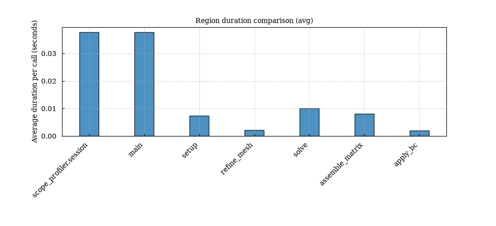
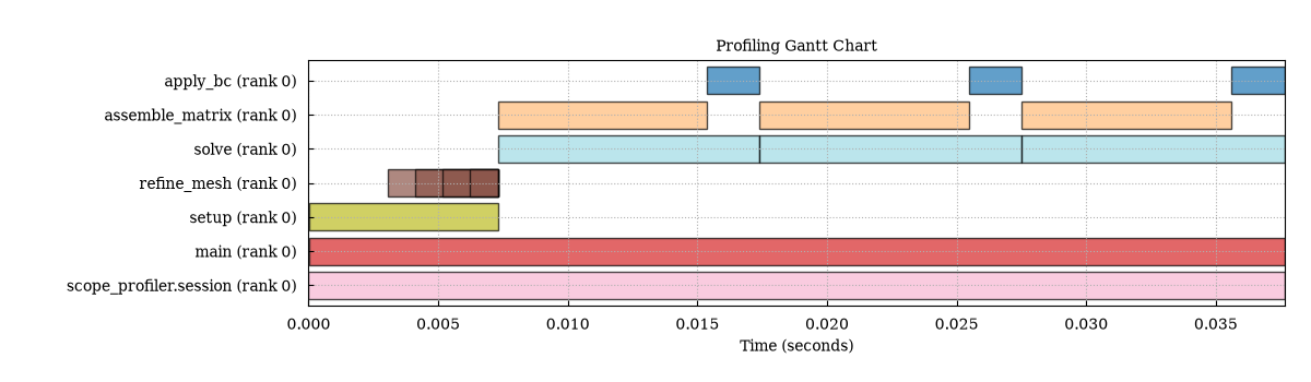
The plotting tools include duration summaries and timelines for finding expensive regions:
For dense traces, the Gantt view supports time windows, duration filtering, call coalescing, and call-depth collapsing. A binned occupancy heatmap avoids drawing every short event:
scope-profiler plot gantt profiling_data.h5 -o figures \
  --min-duration 0.001 --aggregate-calls 25 --collapse-depth 2
scope-profiler plot density profiling_data.h5 -o figures \
  --bins 200 --min-duration 0.0001 --start-time 0 --end-time 10
Use --aggregation-mode with scope-profiler run when only aggregate
timing statistics are needed and the per-call timeline should not be
recorded.
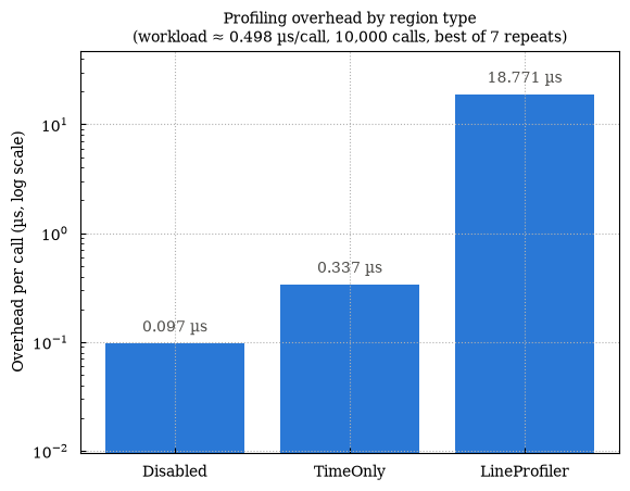
The overhead benchmark measures the cost of each instrumentation mode:
python examples/benchmark_overhead.py
In a notebook
%load_ext scope_profiler.ipython_magics adds magics for the
measure/compare loop, so a notebook needs no session() boilerplate:
%%scope_recursive
result = solve(problem)     # every call recorded, nothing instrumented
%scope_compare baseline candidate
%%scope times a cell as one region, %%scope_line breaks a function
down by line, %%scope_agg handles regions entered millions of times,
and %scope_load pulls in an HDF5 run from an MPI job to compare
against. See the notebook magics
guide.
pip install "scope-profiler[notebook]"
Documentation
- Installation
- Quick start
- Python API and post-processing
- CLI reference
- Plotly figures for the web
- Configuration and profiling regions
- MPI, C, and Fortran
- LIKWID, line profiling, and MCP
- Jupyter/IPython magics
- Tutorial notebooks
- Examples
Build the documentation locally
The hosted documentation is built with Sphinx from the .qmd sources.
Install Quarto and Pandoc first,
then create a development environment and run the docs target from the
repository root:
python -m venv .venv
source .venv/bin/activate
python -m pip install --upgrade pip
pip install -e ".[docs]"
make -C docs html
This refreshes the generated command output and Markdown sources before
building the HTML site. Open docs/build/html/index.html locally, or
serve that directory with any static-file server. The GitHub Pages
workflow uses the same make -C docs html command.
Development
pip install -e '.[dev]'
pytest
See AGENTS.md for the measured benchmark workflow used when optimizing this project.
1 maintainer

Metadata
1 maintainer
Release files for scope-profiler 0.5.1
For a detailed explanation of source distributions (sdists) and built distributions (wheels), please see the package formats documentation.
Source distribution (sdist)
| File | Size | Uploaded | |
|---|---|---|---|
| scope_profiler-0.5.1.tar.gz | 452.0 kB | Details |
Built distribution (wheel)
| File | Interpreter | ABI | Platform | Reset |
|---|---|---|---|---|
| scope_profiler-0.5.1-py3-none-any.whl | Python 3 | none | any | Details |
Total release size: 965.8 kB
Release files / scope_profiler-0.5.1.tar.gz
| Download URL | scope_profiler-0.5.1.tar.gz |
|---|---|
| Size | 452.0 kB |
| Tags | Source |
|
SHA-256 checksum How to use checksums |
edef670f404a09e3a3510c2ba8d9289832f7c4522c15861c628abd75ac170702
|
|
BLAKE2b-256 checksum How to use checksums |
0aa2664bb168153b01f5094800eceb588c81567f1dbeaac471ad0f7874cac009
|
| Upload date | |
|
Uploaded using Trusted Publishing? What is trusted publishing? |
Yes |
| Uploaded via |
twine/7.0.0 CPython/3.13.14
|
Provenance
Provenance describes where a file came from. On PyPI, provenance is shared via attestations, which provide a verifiable record of the build or publishing details. View details, limitations and caveats.


PyPI Publish Attestation
PyPI verified that this artifact, at this checksum, originated from the publisher listed below.
Signed by GitHub Actions, verified by PyPI on Sep 3, 2026.
Transparency logRelease files / scope_profiler-0.5.1-py3-none-any.whl
| Download URL | scope_profiler-0.5.1-py3-none-any.whl |
|---|---|
| Size | 513.8 kB |
| Tags | Python 3 |
|
SHA-256 checksum How to use checksums |
bb62d27b46a30431d55669a1fb9d6470d98e684503497b0eb57b8435285bbfa0
|
|
BLAKE2b-256 checksum How to use checksums |
ea85331cd60fca9077deff5d6dd747dd4e3c112fde2d3830a1bc76de60349dd6
|
| Upload date | |
|
Uploaded using Trusted Publishing? What is trusted publishing? |
Yes |
| Uploaded via |
twine/7.0.0 CPython/3.13.14
|
Provenance
Provenance describes where a file came from. On PyPI, provenance is shared via attestations, which provide a verifiable record of the build or publishing details. View details, limitations and caveats.
PyPI Publish Attestation
PyPI verified that this artifact, at this checksum, originated from the publisher listed below.
Signed by GitHub Actions, verified by PyPI on Sep 3, 2026.
Transparency log













