
Segfix

A GUI tool to fix the instance segmentation of tree point clouds. Load a segmented LiDAR cloud, see each tree in its own colour, and correct mistakes by lassoing points and reassigning, splitting off, or dismissing them, then save back to a corrected version of the input, retaining all fields.
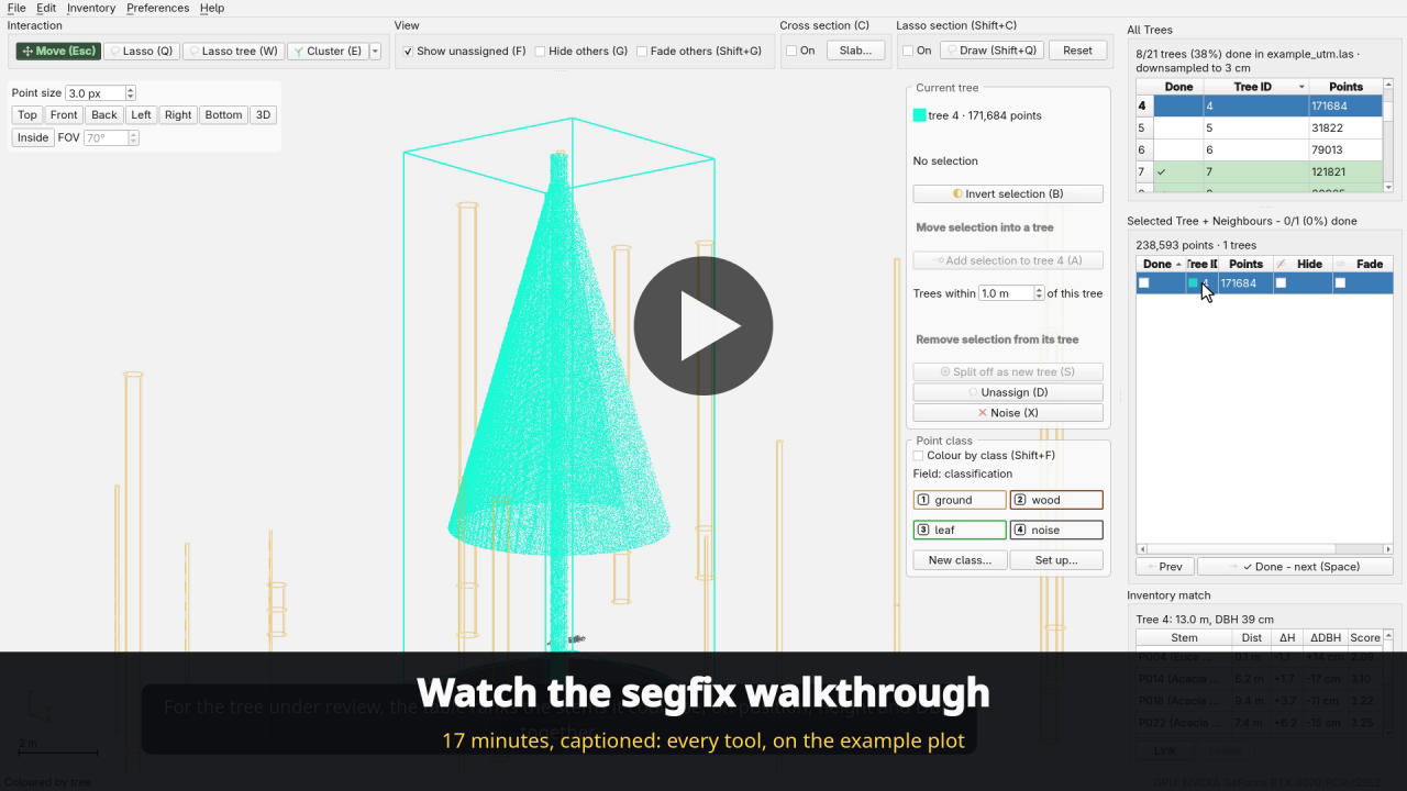
Walkthrough video
A 17-minute captioned tour of every tool, fixing every tree in the example
plot from scripts/make_sample.py: large coordinates and dense clouds, the
editing loop, leaf and wood classes, and matching a field stem map. Click to
watch:
Testing is done on Fedora Linux 44, Windows 11 and macOS.
Contributing
Feedback, issues, and PRs all welcome. For issues please use GitHub issues (not a personal message) so the community can benefit.
Install
Requires Python 3.10–3.12. The package is on PyPI: pypi.org/project/segfix.
pip install segfix
The startup dialog tells you when a newer release is on PyPI, and its
Update… button runs pip install --upgrade for you (restart Segfix
afterwards). On Windows, which can't replace a program while it runs, Segfix
closes first and the update installs in its own window; start Segfix again
when that window says it's done. Running from a clone instead, it tracks new commits on the branch
you're on and updates with git pull + pip install -e ., so a development
checkout stays a checkout.
Using a dedicated environment:
conda create -n segfix python=3.11
conda activate segfix
pip install segfix
From source
For development, or to get scripts/make_sample.py:
git clone https://github.com/UQ-EORC/Segfix.git
cd segfix
pip install -e .
On Windows
Two ready-made builds on the releases page, neither needing admin and neither needing Python:
The installer, segfix-<version>-setup.exe: installs per-user by
default (all-users only if you have the rights), adds a Start Menu entry and
an uninstaller. Being unsigned, Windows shows a SmartScreen warning the
first time: More info → Run anyway.
The portable zip, segfix-<version>-portable.zip: unzip anywhere and
run segfix.exe from the folder. Nothing is written outside it.
Both bundle their own Python, Qt, numpy and scipy, including Qt's software
OpenGL fallback for machines without a usable graphics driver. If a managed
machine refuses to run either (some block unsigned executables outright),
pip install segfix into an existing Python still works, as above.
Run
segfix
segfix will open a startup dialog. Double-click a recent project to reopen
it, or start a new one: New Project… imports a single point cloud, and
New from Per-tree Files… imports a set of one-cloud-per-tree files, merged
into one on the way in (see Per-tree files).
Either way the data is copied into a new project folder (created inside the
directory you pick, named after the source) and that copy is opened, edits are
always saved to the copy, never the original source file.
Every project opened this way is recorded in ~/.config/segfix/registry.json
(a plain JSON file) so it shows up in the "Recent projects"
list next time, most-recently-opened at the top and preselected, each row
showing how long ago it was last opened.
The per-point tree ID field is auto-detected (treeID, PredInstance,
label, …); override with --label-field NAME if needed. Labels that can't
be a real tree ID, negatives (other than the noise marker) and values that
overflow a signed 32-bit int, both of which some pipelines use as a "no tree"
sentinel, are folded into unassigned on load, so they don't show up as
spurious trees.
Accepted formats
Binary PLY, RGB-segmented (raycloudtools) or with a label field, and
LAS. Both store their points as fixed-size records at a known offset, which
is what lets treecatalog.py memory-map a whole plot, read back just the points
of one tree, and on save patch only the label bytes that changed.
raycloudtools output
raycloudtools' rayextract trees writes <plot>_segmented.ply, a binary PLY with no label column, each
point instead coloured by tree (x y z time nx ny nz red green blue alpha,
double xyz). Segfix detects the RGB encoding, maps each distinct colour to a
tree, and treats pure black (0, 0, 0) as unsegmented. Import the .ply
directly; Save patches the colour bytes of points whose tree changed, in
place, so the file stays in exactly the format rayextract produced.
One caveat: noise (X) and unassigned points are both written back as black,
so once such a file is reloaded the two are indistinguishable (Segfix's
.segfix.json sidecar still remembers which were noise for the current
project). New trees created during editing (S, splits) get a deterministic
colour derived from their id.
Sylva output
Sylva's sylva trees --segment writes
<cloud>_segmented.laz (or .ply) with a per-point tree_id column: trees
numbered from 1, and -1 for every point no stem claimed. Segfix finds
tree_id on its own, so the file opens as it is.
Segfix writes -1 for a point it has dismissed as noise, so the first
time it opens a cloud with -1 labels it asks what they mean there:
Unassigned (Sylva, and most other segmentation tools) or Noise
(a cloud Segfix saved, opened without its project folder). The answer is
remembered with the project, and whichever way it was read, -1 is what
goes back to the file on save: Sylva reads 0 as a tree numbered zero, so
unassigned has to go home the way it arrived. Which points you dismissed as
noise stays in Segfix's own .segfix.json sidecar, since the file has only
one way to say "no tree".
So a Sylva plot needs nothing done to it:
sylva trees --segment plot.laz      # writes plot_segmented.laz
segfix                              # open it, answer "Unassigned", fix, save
Sylva's other two columns are useful here as well. classification from its
ground filter (ASPRS codes, 2 = ground) is a class field Segfix can edit
directly, so leaf/wood labels from sylva.leaves can be corrected in the
same pass as the tree IDs (see Point classes), and
sylva.trees stem positions and DBH make a stem map for
inventory matching.
arbor output
arbor's pipeline (arbor segment …) writes
<plot>_output/<plot>_segmented.laz, a point cloud with a per-point treeID
Extra-Bytes column (0 = unassigned). Import that .laz directly: Segfix
decompresses it to a .las working copy in the project folder (the original
.laz is never touched), you fix the treeIDs with the workflow below, and
Save patches the .las in place and re-compresses a fresh .laz beside
it for arbor to re-read.
One caveat: if a cloud's treeID column is an unsigned type, points you
dismiss as noise (X) are written back as 0 (unassigned), Segfix's own
.segfix.json sidecar still remembers they were noise, but a reader of the LAS
alone cannot tell noise from unassigned. (arbor writes a signed treeID, so
this does not apply to its output.)
Per-tree files (one cloud per tree)
Plenty of pipelines emit one file per tree, such as raycloudtools'
raysplit and most per-tree extraction tools, usually with a ground or
unassigned cloud beside them. New from Per-tree Files… on the startup dialog imports such a set
directly:
pick the files (or a whole folder), and Segfix merges them into one project
cloud with each file's tree ID written per point, leaving the originals
untouched.
Which file is which tree is decided before anything is merged, and the table shows the answer for every file as you change it:
- from the filename, by a regular expression you can edit, defaulting to
the last run of digits, so
plot12_tree_7.plyis tree 7; - from a mapping CSV of
path,tree_idrows, which wins over the filename wherever it has a row (matched on the full path or just the name); - typed in for a one-off file, in the Tree ID column;
- as ground: tick Ground and that file's points come in as unassigned rather than as a tree. More than one is fine.
Import is refused until every file has an ID, and if two files claim the same tree. The merged copy keeps the fields every input has (LAS: the first file's point format, with offsets covering the whole set; PLY: the properties common to all of them), and any tree-ID column already in a file is ignored: the filename is the authority, which is the point of importing this way. Export Trees… writes the set back out one file per tree, under those same IDs.
This is worth preferring to merging the files yourself: a merged cloud with no tree-ID field falls back to numbering trees by their RGB colour, which has nothing to do with the numbering your segmentation used.
Field inventory (stem map) matching
Inventory ▸ Load Stem Map… reads a field stem map (a CSV of measured trees), draws each one over the cloud as a wireframe cylinder of its DBH and height, and ranks the likely matches for the tree under review.
Columns are detected by name (tree id/stem/tag, x/easting,
y/northing, dbh/diameter, height, species); DBH in centimetres is
recognised and converted. Rows without usable coordinates are skipped, so a
blank line or a totals row costs nothing.
Alignment. A stem map is rarely in the cloud's coordinates: it may be in a local plot frame, or global but measured with a handheld GPS. Segfix fits the shift from the pattern of stems (every stem-to-tree offset votes, and the winning one is refined), which survives the trees that only one of the two has, and a plot-local map against a UTM cloud is just a large shift. The dialog reports it in metres ("10 stems within reach · median 0.74 m"), and X and Y can be nudged by hand with the cylinders moving as you type.
Candidates. For the tree under review, the Inventory match table ranks stems by position, height and DBH together, best first. Position alone is ambiguous in a closed stand, where the nearest stem is routinely the wrong one. The tree's height comes from its points, and its DBH from a circle fitted to a slab at breast height; a fit that isn't round enough to trust (one side of a trunk, a fork) is shown with "poor fit" and left out of the scoring rather than allowed to rank the wrong stem first. The score is 0 for a perfect match, and roughly 1 at the edge of tolerance. Selecting a row lights that cylinder up in the view, so a ranking can be checked against the trunk rather than taken on trust.
To try it without field data, scripts/make_test_set.py writes a set of
synthetic plots with matching inventory: an open plot, a closed canopy
where the nearest stem is often the wrong one, a 15° slope, leaning stems,
and a georeferenced plot that also triggers the large-coordinate and dense
prompts. Each comes with the truth it was built from and two stem maps (one
plot-local), and --check scores the matching against that truth:
python scripts/make_test_set.py ~/segfix_test_data --check
For a cloud you already have, scripts/make_stem_map.py writes a synthetic
stem map for it, with the errors that make matching real work: positions metres out, optionally in a local plot frame, heights a
few per cent off, trees the crew missed and stems the scan never saw.
python scripts/make_stem_map.py plot.las stems.csv --local --jitter 1.0
Matching needs the cloud's coordinates near the origin: they are held as 32-bit floats, so a raw UTM northing is kept only to about half a metre, which is coarser than the stem positions and the circle fit are built out of. Loading a stem map against an unshifted georeferenced cloud says so; reopen and accept the global shift.
Link (or double-click a row) records the match: the cylinder turns green,
the link is saved in the project's .segfix.json sidecar beside the Done
list, and that stem drops out of every other tree's candidates: one stem,
one tree. Inventory ▸ Export Matches… writes the whole plot as
tree_id,stem_id,species,matched_by,distance_m,height_diff_m,dbh_diff_m,score,…,
with the trees you linked by hand marked manual and the rest filled in by a
greedy one-to-one matching marked auto.
Large coordinates
Georeferenced clouds (UTM, State Plane, …) have coordinates in the millions, while the detail that matters for fixing a segmentation is sub-metre. Segfix stores coordinates as 32-bit floats, as the GPU does, and a float32 carries only about 7 significant digits: a northing around 7,000,000 m is kept to the nearest half metre.
So when any coordinate is more than 10 km from the origin, Segfix offers a global shift on load, the way CloudCompare does: a round offset, added to every coordinate, that brings the cloud near the origin. The suggested shift puts the cloud's minimum corner within a metre of the origin; you can edit X, Y and Z before choosing Apply Shift, or choose Keep Original Coordinates.
The shift applies to this session only. Nothing is written back: Save patches only the label (or, for RGB-segmented PLY, colour) bytes, so the file keeps its real, georeferenced coordinates byte for byte.
If you keep the original coordinates, the cloud loads with that lost precision, and Segfix skips the dense-cloud check below: a spacing measured on coordinates rounded to half a metre would be meaningless, so it won't offer to downsample.
Dense clouds
On load Segfix measures the cloud's typical point spacing. If points are closer than 2 cm it offers to downsample for the session, one point per voxel (3 cm by default, editable in the prompt), which is plenty to see and re-label a tree but a fraction of the points to draw and lasso. The prompt shows what the size you pick would actually keep ("keeps about 42% of the points (204,207,954)"), measured from sample boxes of the cloud and updated as you change the size. Worth reading before accepting: how much a voxel thins a cloud depends on how its points are spread, not on the average spacing, and a cloud measuring 1.7 cm can still keep 85% of its points at 3 cm. Choose Keep Full Resolution and nothing changes.
Downsampling is a working-set choice, not a destructive one. Nothing is written until you save, and on Save the labels you edited are interpolated back onto every original point: each full-resolution point follows the nearest kept point that was the same tree as it, and only where that kept point is one you actually re-labelled, so untouched parts of the cloud keep their original labels byte for byte. The saved file has all of its points and all of its fields, in the format it came in.
The one thing to know is that a voxel is the resolution limit while you work: where two trees' points share a voxel, one label represents it, and unassigned points that fall inside a tree's voxels aren't separately selectable until you reload at full resolution. Pick a voxel smaller than the detail you need to separate. Edits that move a whole tree (X or U on the current tree, a complete merge) still reach every one of its original points, including any in voxels where another tree's or the ground's point was the one kept.
Editing workflow
The menu bar carries the session-level actions: File ▸ Open Project…
(Ctrl+O, reopens the startup dialog and switches project without a manual
restart), Save Project (Ctrl+S) and Export Trees…; Edit ▸ Undo / Redo (Ctrl+Z /
Ctrl+Shift+Z); Inventory ▸ Load Stem Map… / Align to Cloud… / Export
Matches… / Clear Stem Map (see
Field inventory matching);
Preferences ▸ Theme ▸ Light / Dark (light on a first run), applied
immediately and remembered (via QSettings) for next launch; and Help ▸ About Segfix
for the version, links, and full GPL licence.
Navigation matches CloudCompare: clouds open Z-up, left-drag rotates, right-drag pans, wheel zooms. Double-click a point while navigating to recentre the orbit on it. A metric scale bar and an X/Y/Z orientation tripod sit in the bottom-left of the view; the point size spinner floats in the top-left, with CloudCompare's standard view buttons below it: Top, Front, Back, Left, Right and Bottom turn the camera to look at that side (Top looks straight down, Front along +Y), and 3D goes back to the tilted view. They only turn the camera, so whatever you're centred on stays in view at the same zoom.
Below the view buttons, Inside stands the camera at a point in the cloud and switches to a perspective projection, like CloudCompare's bubble view. An orthographic view of a dense plot is a wall: every stem at every distance is drawn the same size, so what is in front of what can't be read, and a crown ten metres behind the one you're editing looks like part of it. From inside, near points spread apart and far ones converge, so a gap you can see through is a gap. Double-click a point to choose where to stand (or to move while you're there), drag to look around, FOV sets how wide the lens is, and scrolling pulls back out. Framing a whole tree, by stepping through the queue or loading another tree, steps back outside on its own.
The right-hand panel holds two tables. All Trees (top) lists every tree in the
file, a Done column (✓ when reviewed), tree ID and point count, with a
running N/M trees (X %) done line above it, double-click a row to load
that
tree plus its spatial neighbours into the 3D view. Selected Tree +
Neighbours (below) is the review queue for what's currently loaded: a Done
checkbox per tree, a 👁 column to hide one from the view, a Fade column to
ghost one (still shown, still selectable), and the Prev / Done buttons. Both
read the same <cloud>.segfix.json sidecar, written next to the working copy,
so a half-finished plot resumes where you left off. Finished rows in either
table get a green tint. The Current tree actions (Add selection,
send-to-neighbour, Split / Unassign / Noise) float as a fixed column pinned
to the right edge of the 3D view, next to the points they act on.
-
Double-click a tree in All Trees. The camera flies to it and a wireframe box marks it. To declutter a crowded view, use the 👁 (hide) or Fade column in the lower table on specific trees, or Hide others / Fade others in the top-bar View group to do it to every loaded tree except the one under review (both stay ticked while they're on, and follow the per-tree columns). Fading keeps a tree visible as faint context and still lets the lasso grab its points; hiding removes it from both.
-
Inspect it. If it's correct, press Space, the tree is marked done, progress is saved, and the next unfinished tree in the loaded set becomes current. That's the loop.
-
If it needs fixing, select points with the lasso: press Q, drag a freehand loop (Shift adds), Esc to go back to navigating. The tree under review is always the implicit target. B inverts the selection when the points you don't want are the easier shape to draw around. Inverting only ever reaches points that are on screen, so a cross section, a lasso section or a hidden tree still bounds it. With nothing selected, B selects everything currently shown.
Key Operation SpaceMark current tree done, jump to next unfinished Z/VPrevious / next tree (without marking done) QLasso select WLasso, but only points already in the current tree, grabs a clean patch out of an overlapping crown ECluster select: click a point to take the connected patch of its tree; click the same spot again to loosen the gap and grow it R/TTighten / loosen the cluster gap one step EscBack to camera / navigation AAdd selection to the current tree (missing branches, unassigned canopy) BInvert the selection, within what's on screen; with nothing selected it takes everything shown 1…5Move selection into a neighbouring tree: the 1st to 5th button under Move selection into a tree, nearest tree first, without switching tree first SSplit selection off as a new tree (it joins the queue unreviewed) DUnassign selection, or the whole current tree if nothing is selected XMark selection as noise, or the whole current tree if nothing is selected (dismiss a bush/wall in one key) Delete/BackspaceSame as X(mark noise)FShow/hide the unassigned + noise points Ctrl+1…Ctrl+5Give the selection the 1st to 5th point class (see Point classes), or the whole current tree if nothing is selected Shift+FColour by point class / by tree G/Shift+GHide / fade every other loaded tree (press again to bring them back) CCross section on/off Shift+QDraw a lasso-section outline Shift+CLasso section on/off Ctrl+Z/Ctrl+Shift+ZUndo / Redo (also on the Edit menu) Ctrl+SSave Project (also on the File menu) Ctrl+OOpen another project Every key sits under the left hand, so the right one never leaves the mouse: the tools on
QWEwith the cluster gap beside them onRT, the edits along the home row, and the queue onZ/V/Space. The keys these replaced (L,Ctrl+L,K,[,],N,U,H,Shift+Land the arrow keys) still work.Cluster (
E) is the other way to select: click a point and it takes the patch of that point's tree that is physically connected to it. How wide a hole still counts as connected is the gap, in multiples of the cloud's point spacing. It starts at 1×, deliberately tight, so a first click is a small seed; click the same spot again to loosen it a step and grow the patch (1× → 1.5× → 2× … up to 16×), or useR/T, or the ▾ beside the Cluster button for a slider. Changing the gap re-runs your last click, so the patch grows or shrinks on screen as you go. The gap goes back to 1× when you switch Cluster off, or when the selection is cleared (afterA/S/D/X, a click on empty space, or moving to another tree).To move stray points to a neighbour instead, lasso them and click one of the → id buttons in the Current tree panel, one per tree within "reach" metres of this one. Clicking that neighbour's table row to make it current and pressing
Adoes the same thing.To merge an over-segmented fragment back in, lasso the whole fragment and press
A; there is no separate merge key.Handing a patch to the tree next door is the commonest fix where two crowns overlap. The Move selection into a tree box lists the current tree's neighbours as coloured buttons, closest first. The nearest five sit at the top and never scroll, each wearing the keycap that presses it (
1…5); any further neighbours scroll in the box below, and are a click away. So the whole correction is lasso, then one key, with the mouse never leaving the canvas and the hand never leaving the keys. Hovering a button says how close that tree comes. Listed above: trees within … m under the buttons is what decides which trees appear there at all. Buttons that need a selection are greyed out until there is one; Unassign and Noise stay live, since with nothing selected they act on the whole current tree. -
For a crowded canopy, two tools in the top bar cut the view down. Both fold into the same visibility as the 👁 column, so hidden points are also unselectable and the lasso can't grab through them:
- Cross section (
C), a slab along X, Y or Z, set with two sliders. - Lasso section (
Shift+C), same idea, but the kept region is an outline you draw (Shift+Q, then drag). It's frozen into a point mask as you release, so the camera moves freely afterwards.
Both reset when a new tree is loaded.
- Cross section (
-
Leftover unassigned points may hide missed trees: they're loaded alongside every tree you open, so lasso one and press
Sto promote it to a tree of its own (it joins the queue unreviewed). -
Save (
Ctrl+S) writes to the project copy, never the original import. It patches only the points whose label changed, in place, so the header and every other column are untouched byte for byte. -
File ▸ Export Trees… writes every tree in the cloud to a folder you pick, one file per tree, named after the cloud (
plot_a.las→plot_a_tree_7.las) and in its format. Each file carries all of that tree's points at full resolution (whole trees even from a downsampled session), with every column and the file's own coordinates, so an exported tree still lands in the right place in any other tool. Unassigned points and anything dismissed as noise aren't trees and aren't written. Trees are exported as the saved file has them, so Segfix offers to save first. If any trees are marked Done it also asks which to write, all of them or only the Done ones, for when a plot is reviewed for the few trees you actually need.
Point classes
Besides which tree each point belongs to, Segfix can edit what each point
is (leaf, wood, understorey, ground, or any classes you use), held in one
numeric per-point field of the cloud, such as a LAS classification or a
PLY property like semantic.
Edit ▸ Point Classes… (or Set up… in the Point class box under
Current tree) picks the field and names its values. The file stores only
numbers, so the names are yours: the dialog lists every value the field
holds, and you type what each one means (a LAS classification starts from
the standard ASPRS names). Add class adds a value the file doesn't have
yet. The field and names are remembered with the project, so they're set
once. --class-field NAME on the command line picks the field too.
Classes are edited inside the same tree-and-neighbours review. The
Point class box has a button per class, the first five on
Ctrl+1…Ctrl+5: lasso some points and press one to give them that class,
or press one with nothing selected to give the whole current tree that class.
Colour by class (Shift+F) colours the points by class instead of by
tree (wood brown, leaves green and ground tan when the names say so), and
a tree's fade still applies. New class… adds a class numbered one above
the rest and gives it to the selection, if there is one. Class edits undo and
redo along with the tree edits, in the order they were made.
The box floats over the 3D view, under Current tree, which on a laptop screen is most of the view. Point class in top bar in the View group moves it into the top strip instead, beside Cross section and Lasso section: the same box with the same buttons, not a second copy. It floats by default, since a project with no class field never needs it.
Save writes only the class values that changed, like the tree IDs, so every other byte of the file stays as it was. In LAS point formats 0–5 the classification is the low five bits of a byte it shares with the synthetic, key-point and withheld flags; only those five bits are written, so values run 0–31 there. On a downsampled session, class edits are carried back to every original point the way tree edits are, each point following the nearest kept point of the same tree and class.
Layout
| File | Responsibility |
|---|---|
model.py |
PointCloud data + undo/redo (diff-based) |
io.py |
whole-cloud load/save (binary PLY, LAS/LAZ), label-field and RGB-segmentation detection |
operations.py |
pure, UI-agnostic label edits (reassign/split/unassign/noise) |
analysis.py |
which trees touch which, by sampled point distance (KD-tree) |
export.py |
File ▸ Export Trees…: one file per tree, full resolution, in the cloud's own format |
density.py |
point-spacing measurement, voxel decimation, and the save-time interpolation back to full resolution |
lasso.py |
3D screen-space lasso (camera projection + polygon test) and the click-to-grow cluster tool |
cloudview.py |
the vispy 3D canvas: camera, points, selection halo, tree box |
viewer.py |
label→colour mapping and visibility masks |
overlays.py |
scale bar + orientation axes painted over the canvas |
theme.py |
light/dark palette, remembered in QSettings |
widgets.py |
Qt dock panel wiring selection → operations |
icons.py |
inline SVG icons for the panel buttons and window |
treecatalog.py |
default mode: memory-mapped tree-label grouping, neighbour load + write-back (TreeCatalog = PLY, LasCatalog = LAS, open_catalog picks) |
scene_ui.py |
tree table + scene controller for the default mode |
shift_ui.py |
load-time "large coordinates" (global shift) prompt |
negative_ui.py |
load-time "what does a tree ID of -1 mean here" prompt |
density_ui.py |
load-time "dense cloud" (downsample) prompt |
progress_ui.py |
progress window for the two slow operations, opening and saving |
registry.py |
on-disk list of recently opened files/projects |
workspace.py |
project folders: copy (or decompress .laz→.las) an imported file, never touch the source |
startup_ui.py |
startup dialog: pick a recent entry or start a new project |
merge.py |
per-tree file sets: filename/CSV → tree ID, and the streamed merge into one project cloud |
multi_import_ui.py |
the per-tree import dialog: which file is which tree |
inventory.py |
field stem maps: CSV → stems, the coordinate fit, candidate ranking, match CSV |
inventory_ui.py |
stem-map loading and the alignment dialog |
classes_ui.py |
Edit ▸ Point Classes…: pick the class field and name its values |
update.py |
update check: a newer PyPI release for an installed copy, new commits for a git checkout |
app.py |
segfix CLI entry point |
Tests
pytest # core model, operations, and IO round-trip (no GUI needed)
Authors
- Tim Devereux, The University of Queensland
- Josh Rivory, The University of Queensland
Development of this software was made possible by funding from The Terrestrial Ecosystem Research Network (TERN).
Citation
If Segfix contributed to your work, please cite it:
Devereux, T. and Rivory, J. (2026). Segfix: a GUI tool to fix the instance segmentation of tree point clouds (version 1.1.0) [Computer software]. The University of Queensland. https://github.com/UQ-EORC/Segfix
@software{segfix,
  author       = {Devereux, Tim and Rivory, Josh},
  title        = {Segfix: a GUI tool to fix the instance segmentation of
                  tree point clouds},
  year         = {2026},
  version      = {1.1.0},
  organization = {The University of Queensland},
  url          = {https://github.com/UQ-EORC/Segfix}
}
1 maintainer

Metadata
1 maintainer
Release files for segfix 1.1.0
For a detailed explanation of source distributions (sdists) and built distributions (wheels), please see the package formats documentation.
Source distribution (sdist)
| File | Size | Uploaded | |
|---|---|---|---|
| segfix-1.1.0.tar.gz | 302.7 kB | Details |
Built distribution (wheel)
| File | Interpreter | ABI | Platform | Reset |
|---|---|---|---|---|
| segfix-1.1.0-py3-none-any.whl | Python 3 | none | any | Details |
Total release size: 523.2 kB
Release files / segfix-1.1.0.tar.gz
| Download URL | segfix-1.1.0.tar.gz |
|---|---|
| Size | 302.7 kB |
| Tags | Source |
|
SHA-256 checksum How to use checksums |
fd5b7308bae8d61e854f90e02f6686c2f571d214253998a5ec6f5e024698d038
|
|
BLAKE2b-256 checksum How to use checksums |
49443615be8141c35066d421394547c0617d5ba2af32463c313ec565143dcecc
|
| Upload date | |
|
Uploaded using Trusted Publishing? What is trusted publishing? |
Yes |
| Uploaded via |
twine/7.0.0 CPython/3.13.14
|
Provenance
Provenance describes where a file came from. On PyPI, provenance is shared via attestations, which provide a verifiable record of the build or publishing details. View details, limitations and caveats.


PyPI Publish Attestation
PyPI verified that this artifact, at this checksum, originated from the publisher listed below.
Signed by GitHub Actions, verified by PyPI on Oct 5, 2026.
Transparency logRelease files / segfix-1.1.0-py3-none-any.whl
| Download URL | segfix-1.1.0-py3-none-any.whl |
|---|---|
| Size | 220.5 kB |
| Tags | Python 3 |
|
SHA-256 checksum How to use checksums |
e230c2d7003cccab549d4bedd82a9d61f194c22e724406e8bfdf4595a2ffc71e
|
|
BLAKE2b-256 checksum How to use checksums |
cb399df28d9c639d728de7e0341764a7c20ee6df8693d13dfc8e666e7ef7932d
|
| Upload date | |
|
Uploaded using Trusted Publishing? What is trusted publishing? |
Yes |
| Uploaded via |
twine/7.0.0 CPython/3.13.14
|
Provenance
Provenance describes where a file came from. On PyPI, provenance is shared via attestations, which provide a verifiable record of the build or publishing details. View details, limitations and caveats.
PyPI Publish Attestation
PyPI verified that this artifact, at this checksum, originated from the publisher listed below.
Signed by GitHub Actions, verified by PyPI on Oct 5, 2026.
Transparency log













