
Starplast
← Back · Next → · Open slide viewer · PDF · PowerPoint

















Starplast is a desktop app for exploring gene evidence in Toxoplasma gondii and Plasmodium falciparum. It brings expression, fitness screens, localization, protein features, interactions, and literature annotations into one place.
Use it to look up a gene, investigate hits from a screen, compare groups of genes, and choose candidates for follow-up experiments. The bundled maps contain 8,140 T. gondii genes and 5,720 P. falciparum genes, viewed separately.
User guide · Python API · Dataset catalogue · Changes
Install
Python 3.10 or newer is required. The desktop app needs a display and OpenGL.
pip install starplast
starplast
From a checkout:
git clone https://github.com/EinarOlafsson/starplast.git
cd starplast
pip install -e .
starplast
The default installation runs analyses on the CPU. For an NVIDIA GPU on Linux x86_64 with a CUDA 12 compatible driver:
pip install "starplast[gpu]"
GPU dependencies are large and optional. starplast-install-gpu can also inspect
your driver and offer an installation command. macOS and Windows use CPU analysis;
the 3D display still uses OpenGL.
The built gene tables and graphs ship with the package. Browsing them works offline. Protein structures are downloaded when requested and cached locally. Rebuilding the bundled data requires the original source datasets.
Explore a screen
- Choose the organism under File → Species.
- Search for a gene ID. For T. gondii, File → Import data adds your screen results.
- Colour and filter the map using the measurements you want to compare.
- Click a gene to read its evidence and inspect each type of relationship separately.
- Select a group with a lasso or brush, then export the gene list for follow-up.
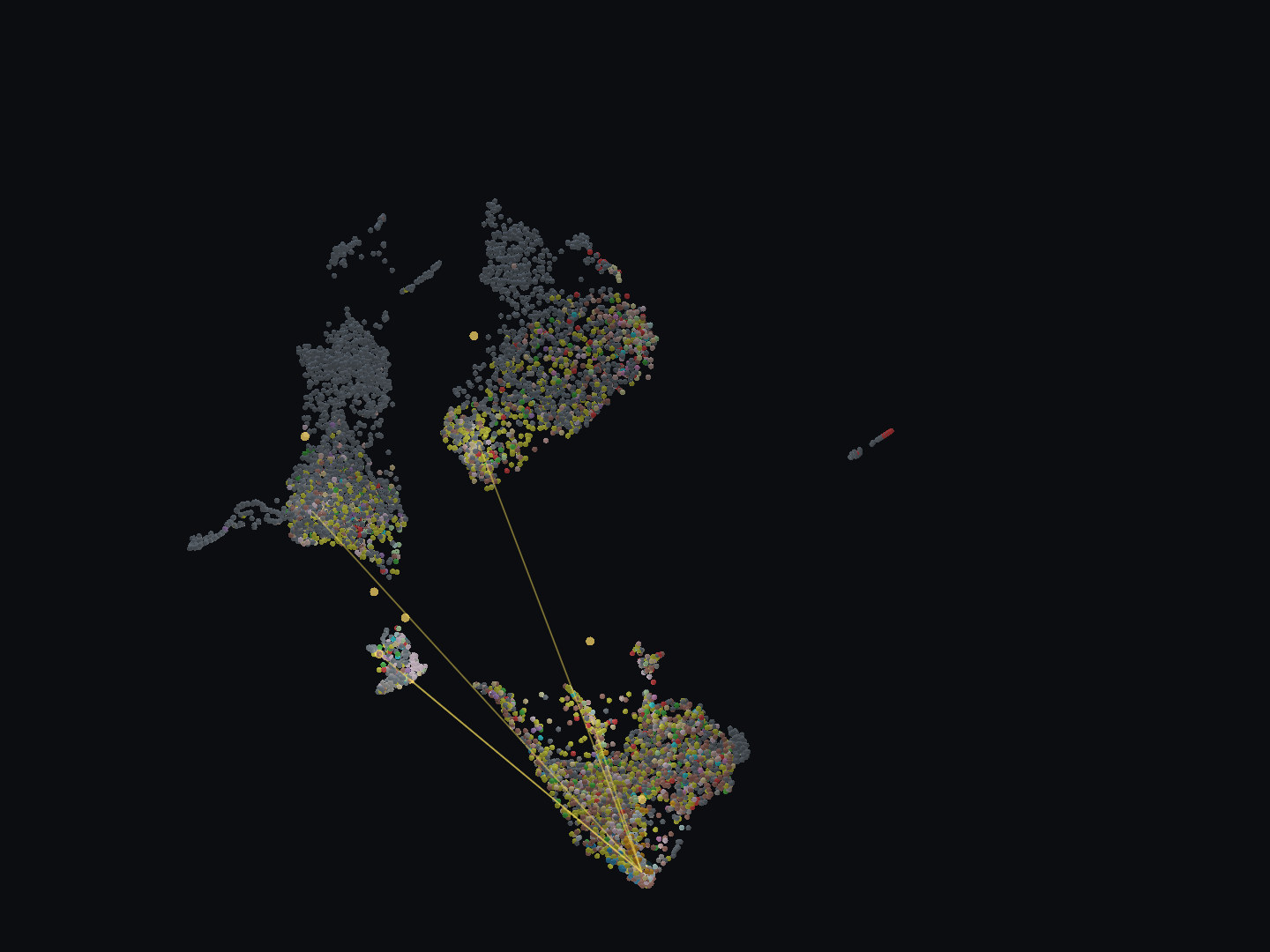
The T. gondii map with CDPK1 (TGME49_301440) selected. The selected gene and
its five neighbours emit light; lines show attention-corrected literature
co-mention links. Colours show compartments. This animation uses the pre-0.43
layout; newly opened maps use the recorded, balanced feature recipe.
View a still image.
Each point is a gene. Its position comes from an embedding of selected features; nearby points have similar inputs, but proximity alone does not demonstrate a shared function or physical interaction. Colours, relationship edges, and the evidence panel provide the context needed to interpret the map. Missing evidence is shown separately from measured values.
The analysis panel lets you change feature sets, build embeddings, cluster genes, and evaluate recovery of labels held out from the input. Search scores help prioritize candidates; they are not experimental validation. See the user guide for controls and analysis settings.
The search box beside the Help menu (Ctrl+Shift+H), as in spaCR, finds any menu command, panel, strategy, setting, slot, dataset or guide section and takes you to it.
Explore, predict and compare
The Tools menu offers three starting points:
- Explore a gene searches identifiers, symbols and descriptions, then shows the source evidence.
- Predict a trait compares held-out predictions before making calls for unlabelled genes. Related genes stay in the same evaluation group; reports retain missing values, calibration status and exact input settings.
- Compare a screen joins a gene-level CSV/TSV to the existing evidence and keeps unresolved identifiers visible.
The package includes frozen protein sequence representations for 8,064 Toxoplasma proteins and AF3 summary features for 1,210 exactly mapped genes. Sequence features are optional inputs to prediction; local structure files can also be indexed for the structure viewer.
In the 0.43 benchmark, boosted trees with sequence and structure features reached 56.2% localization accuracy across held-out orthogroups. UMAP neighbours performed less well, and several rare classes remained poorly recovered. These are model hypotheses, not experimentally established annotations.
Strategies
The strategies tab, beside Evidence and Analysis, lists 39 named ways of turning the combined data into a claim -- from holding a category out and searching for the map that finds it, to calling genes with a stated error rate (conformal prediction) or learning how far to trust each kind of evidence (stacking). Each name ends with its method, such as (UMAP + HDBSCAN); each lists the techniques it is built from, has a guide and a walkthrough, and carries a self-test that hides known information, asks for it back and compares the answer with the same procedure on shuffled data. Every test reports a scorecard: the standard metrics for its kind of task, in a fixed order, so strategies doing the same thing can be compared number by number. The start here tab beside it asks what you have instead -- a gene, a gene list, your own screen, a label, or nothing yet -- one question at a time, and ends at the three to six strategies worth running for that answer, ranked by their grade on that organism and with their settings already filled in.
Measured 2026-09-26 over 7,640 self-tests: every strategy's self-test run over a grid of its settings, several held-out known labels and five seeds. Skill puts every metric on one scale -- 0 is the same procedure on shuffled data, 1 is perfect. Tuned is the best setting chosen on seeds 1-3 and reported on seeds 4-5, so it is not the luckiest of many settings. Intervals are 95%, by bootstrap over held-out targets and runs. Every number, per target and per setting.
T. gondii -- 30 reliable, 8 weak, 1 untestable
| # | Strategy | Metric | Grade | Skill at defaults [95% CI] | Pass | Skill tuned [95% CI] | Pass | Tuned setting | Tests |
|---|---|---|---|---|---|---|---|---|---|
| 01 | Hold out a category and search for a map that finds it (UMAP + HDBSCAN) | F1 of hidden genes in the cluster chosen for their label on known genes | weak | 0.07 [0.03, 0.11] | 44% | 0.07 [0.03, 0.11] | 40% | min_cluster_size=[10, 25]; n_neighbors=[25, 100]; selection=[eom, leaf] | 150 |
| 02 | Find the map where your gene list is one cluster (UMAP + HDBSCAN) | F1 of the hidden members against the best cluster's other genes | weak | 0.03 [0.00, 0.04] | 16% | 0.03 [0.00, 0.05] | 10% | min_cluster_size=[20, 50]; n_neighbors=[10, 30] | 100 |
| 03 | Ask which categories the data can rediscover (UMAP + neighbour AUROC) | hidden-gene AUROC of the categories the atlas ranks in its top half | reliable | 0.50 [0.22, 0.68] | 80% | 0.50 [0.22, 0.68] | 80% | k=15 | 75 |
| 04 | Keep only the modules that survive the whole walk (UMAP + HDBSCAN co-clustering) | F1 of hidden genes in the module chosen for their label on known genes | weak | 0.07 [0.01, 0.13] | 56% | 0.05 [-0.04, 0.10] | 50% | threshold=0.3 | 75 |
| 05 | Tune a map without labels, then read what it encodes (UMAP + HDBSCAN, chi-square / Kruskal-Wallis) | share of first-half findings that replicate on the second half | reliable | 0.95 [0.88, 1.00] | 100% | 0.96 [0.95, 0.98] | 100% | map_from=chemistry | 70 |
| 06 | Find which kind of evidence carries a label (kNN ablation) | hidden accuracy of the evidence ranked first (transcription) | reliable | 0.14 [0.06, 0.25] | 64% | 0.16 [0.08, 0.25] | 70% | k=5 | 75 |
| 07 | Call a gene by the genes that behave like it (kNN) | correct calls per hidden gene | reliable | 0.22 [0.08, 0.36] | 60% | 0.29 [0.16, 0.43] | 80% | k=5; min_share=0.0 | 225 |
| 08 | Call a gene by its neighbours on the map (UMAP + kNN) | correct calls per hidden gene | weak | 0.13 [0.01, 0.24] | 60% | 0.11 [-0.04, 0.23] | 60% | k=5; n_neighbors=60 | 225 |
| 09 | Name a cluster by the label it is enriched for (UMAP + HDBSCAN, hypergeometric) | precision of calls on hidden genes | reliable | 0.33 [0.25, 0.42] | 100% | 0.41 [0.30, 0.50] | 100% | min_cluster_size=10; min_lift=3.0; selection=leaf | 300 |
| 10 | Find genes whose label their neighbours contradict (kNN + network neighbours) | AUROC of surprise for the swapped labels | reliable | 0.64 [0.49, 0.77] | 100% | 0.65 [0.51, 0.78] | 100% | k=15 | 75 |
| 11 | Diffuse a label across one measured network (random walk with restart) | correct calls per hidden gene | reliable | 0.12 [0.08, 0.17] | 75% | 0.14 [0.10, 0.18] | 88% | layer=coexpression; restart=0.2 | 900 |
| 12 | Let every network vote, weighted by what it has earned (chance-weighted ensemble vote) | correct calls per hidden gene | weak | 0.30 [-0.03, 0.54] | 80% | 0.25 [-0.21, 0.54] | 80% | k=15 | 75 |
| 13 | Place a protein by the proteins it physically touches (weighted partner vote) | correct calls per hidden gene | reliable | 0.25 [0.08, 0.43] | 60% | 0.26 [0.08, 0.43] | 60% | -- | 25 |
| 14 | Annotate function through shared fold (TM-score-weighted vote) | correct calls per hidden gene | reliable | 0.64 [0.60, 0.66] | 100% | 0.71 [0.71, 0.72] | 100% | level=3 | 15 |
| 15 | Find the communities several networks agree on (modularity + Louvain consensus) | F1 of hidden genes in the community chosen for their label on known genes | weak | 0.05 [0.02, 0.08] | 40% | 0.05 [-0.00, 0.09] | 40% | agreement=0.5; resolution=1.0 | 150 |
| 16 | Predict the contacts an interactome missed (logistic regression) | AUROC of hidden pairs against degree-matched non-pairs | reliable | 0.61 [0.59, 0.62] | 100% | 0.93 [0.92, 0.93] | 100% | layer=struct | 10 |
| 17 | Read the literature for biology, not fame (publication-count residual) | share of the top 50 corrected pairs sharing a compartment label | reliable | 0.38 [0.21, 0.54] | 80% | 0.38 [0.21, 0.55] | 80% | top=200 | 75 |
| 18 | List what the data says and the literature has not written (multi-layer support count) | AUROC of hidden pairs against random non-pairs | reliable | 0.11 [0.11, 0.11] | 100% | 0.11 [0.11, 0.11] | 100% | min_layers=1 | 15 |
| 19 | Train a classifier on the known genes and call the rest (logistic regression) | correct calls per hidden gene | reliable | 0.32 [0.18, 0.46] | 80% | 0.37 [0.20, 0.50] | 80% | C=10.0 | 100 |
| 20 | Learn what makes your list special, from positives alone (PU bagging, logistic regression) | AUROC of hidden members against every other gene | reliable | 0.79 [0.72, 0.85] | 100% | 0.80 [0.74, 0.85] | 100% | bags=5 | 75 |
| 21 | Predict a measurement, and find the genes that defy the prediction (gradient boosting / ridge) | rank correlation of predicted and hidden values | reliable | 0.56 [0.05, 0.91] | 67% | 0.67 [0.15, 0.97] | 100% | model=boosted; own_kind=include | 60 |
| 22 | Fill in what was never measured, and say where that is honest (soft-impute, low-rank SVD) | median per-column rank correlation on hidden entries | reliable | 0.87 [0.86, 0.87] | 100% | 0.90 [0.90, 0.90] | 100% | rank=60 | 15 |
| 23 | Find what matters more in one condition, and why (residual + gradient boosting / ridge) | rank correlation of predicted and hidden values | weak | 0.07 [0.06, 0.09] | 0% | 0.07 [0.05, 0.08] | 0% | model=ridge; own_kind=include | 20 |
| 24 | Describe what your gene list has in common (hypergeometric + rank-sum) | AUROC of hidden members against every other gene | reliable | 0.61 [0.51, 0.72] | 100% | 0.64 [0.52, 0.75] | 100% | -- | 25 |
| 25 | Grow your gene list along the networks (random walk with restart) | AUROC of hidden members against every other gene | reliable | 0.59 [0.49, 0.68] | 100% | 0.61 [0.53, 0.67] | 100% | mode=networks + measurements; restart=0.6 | 150 |
| 26 | Find categories that split in two on another measurement (UMAP + HDBSCAN) | share of findings that replicate | untestable | -- | -- | -- | -- | -- | 15 |
| 27 | Find kinds of gene defined by two labels at once (UMAP + HDBSCAN) | share of first-half findings that replicate on the second half | reliable | 0.49 [0.38, 0.62] | 100% | 0.53 [0.32, 0.74] | 100% | min_cluster_size=15 | 15 |
| 28 | Find paralogs that changed jobs (profile correlation) | AUROC of profile divergence for paralogs with different compartment | reliable | 0.16 [0.06, 0.31] | 60% | 0.16 [0.06, 0.31] | 62% | min_shared=10 | 75 |
| 29 | Carry what one parasite shows to the other (orthogroup mapping) | rank correlation of transferred and hidden values | reliable | 0.31 [0.30, 0.33] | 100% | 0.32 [0.29, 0.35] | 100% | -- | 5 |
| 30 | Test inference on the genes orthology cannot reach (kNN) | correct calls per hidden gene | reliable | 0.26 [0.15, 0.34] | 75% | 0.28 [0.17, 0.36] | 75% | stratum=lineage-specific | 100 |
| 31 | Call a gene only when independent strategies agree (kNN + logistic + network vote) | precision of calls on hidden genes | reliable | 0.35 [0.17, 0.48] | 60% | 0.61 [0.33, 0.77] | 80% | min_agree=3 | 75 |
| 32 | Put the understudied genes first (kNN + logistic + network vote) | precision of calls on hidden genes | reliable | 0.32 [0.13, 0.46] | 60% | 0.59 [0.32, 0.75] | 80% | min_agree=3 | 75 |
| 33 | Put every layer into one space and read a gene's neighbourhood (logistic edge model) | AUROC of hidden coexpression edges against degree-matched non-pairs | reliable | 0.59 [0.58, 0.59] | 100% | 0.90 [0.86, 0.94] | 100% | k=10; knn=15; layer=cotranslation | 150 |
| 34 | Train on the networks and rank the edges they are missing (logistic / spectral embedding) | AUROC of hidden coexpression edges against degree-matched non-pairs | reliable | 0.59 [0.58, 0.59] | 100% | 0.88 [0.88, 0.88] | 100% | fraction=0.4; layer=cotranslation; model=logistic | 100 |
| 35 | Call genes with a stated error rate (split conformal prediction) | set efficiency: 1 - (mean set size - 1) / (classes - 1) | reliable | 0.50 [0.21, 0.73] | 80% | 0.50 [0.20, 0.76] | 80% | alpha=0.2; model=kNN | 150 |
| 36 | Smooth the measurements along the networks, then classify (graph convolution + logistic regression) | correct calls per hidden gene | reliable | 0.40 [0.16, 0.57] | 80% | 0.40 [0.18, 0.56] | 80% | C=0.5; hops=1 | 150 |
| 37 | Let a random forest find what defines a label (random forest + permutation importance) | correct calls per hidden gene | reliable | 0.45 [0.22, 0.65] | 80% | 0.45 [0.21, 0.66] | 80% | min_leaf=5; trees=300 | 150 |
| 38 | Learn how much to trust each kind of evidence (stacked logistic regression) | correct calls per hidden gene | reliable | 0.41 [0.18, 0.57] | 80% | 0.41 [0.20, 0.56] | 80% | k=10 | 75 |
| 39 | Predict a value with an interval that holds (gradient boosting / ridge + split conformal) | rank correlation of predicted and hidden values | weak | 0.55 [0.04, 0.91] | 67% | 0.53 [0.03, 0.86] | 67% | alpha=0.2; model=ridge | 60 |
P. falciparum -- 26 reliable, 9 weak, 2 untestable, 2 works when tuned
| # | Strategy | Metric | Grade | Skill at defaults [95% CI] | Pass | Skill tuned [95% CI] | Pass | Tuned setting | Tests |
|---|---|---|---|---|---|---|---|---|---|
| 01 | Hold out a category and search for a map that finds it (UMAP + HDBSCAN) | F1 of hidden genes in the cluster chosen for their label on known genes | weak | 0.09 [0.01, 0.19] | 25% | 0.11 [0.02, 0.29] | 25% | min_cluster_size=[20, 50]; n_neighbors=[10, 30]; selection=[eom, leaf] | 120 |
| 02 | Find the map where your gene list is one cluster (UMAP + HDBSCAN) | F1 of the hidden members against the best cluster's other genes | reliable | 0.21 [0.09, 0.35] | 90% | 0.22 [0.08, 0.35] | 75% | min_cluster_size=[20, 50]; n_neighbors=[15, 50] | 80 |
| 03 | Ask which categories the data can rediscover (UMAP + neighbour AUROC) | hidden-gene AUROC of the categories the atlas ranks in its top half | reliable | 0.69 [0.56, 0.79] | 100% | 0.65 [0.55, 0.72] | 100% | k=15 | 60 |
| 04 | Keep only the modules that survive the whole walk (UMAP + HDBSCAN co-clustering) | F1 of hidden genes in the module chosen for their label on known genes | weak | 0.15 [0.03, 0.28] | 45% | 0.19 [0.05, 0.39] | 50% | threshold=0.5 | 60 |
| 05 | Tune a map without labels, then read what it encodes (UMAP + HDBSCAN, chi-square / Kruskal-Wallis) | share of first-half findings that replicate on the second half | reliable | 0.88 [0.82, 0.93] | 100% | 0.95 [0.91, 1.00] | 100% | map_from=isoelectric | 250 |
| 06 | Find which kind of evidence carries a label (kNN ablation) | hidden accuracy of the evidence ranked first (expr) | reliable | 0.13 [0.07, 0.19] | 65% | 0.14 [0.08, 0.20] | 75% | k=5 | 60 |
| 07 | Call a gene by the genes that behave like it (kNN) | correct calls per hidden gene | weak | 0.08 [-0.37, 0.42] | 50% | 0.22 [0.02, 0.42] | 50% | k=15; min_share=0.3 | 180 |
| 08 | Call a gene by its neighbours on the map (UMAP + kNN) | correct calls per hidden gene | weak | -0.00 [-0.53, 0.29] | 60% | 0.15 [0.03, 0.27] | 62% | k=50; n_neighbors=25 | 180 |
| 09 | Name a cluster by the label it is enriched for (UMAP + HDBSCAN, hypergeometric) | precision of calls on hidden genes | reliable | 0.42 [0.33, 0.60] | 100% | 0.56 [0.45, 0.70] | 100% | min_cluster_size=25; min_lift=1.5; selection=leaf | 240 |
| 10 | Find genes whose label their neighbours contradict (kNN + network neighbours) | AUROC of surprise for the swapped labels | reliable | 0.74 [0.57, 0.92] | 100% | 0.77 [0.61, 0.92] | 100% | k=15 | 60 |
| 11 | Diffuse a label across one measured network (random walk with restart) | correct calls per hidden gene | reliable | 0.22 [0.14, 0.33] | 93% | 0.24 [0.13, 0.44] | 100% | layer=coexpression; restart=0.2 | 480 |
| 12 | Let every network vote, weighted by what it has earned (chance-weighted ensemble vote) | correct calls per hidden gene | reliable | 0.51 [0.41, 0.65] | 65% | 0.50 [0.39, 0.61] | 62% | k=15 | 60 |
| 13 | Place a protein by the proteins it physically touches (weighted partner vote) | correct calls per hidden gene | weak | 0.22 [0.01, 0.47] | 33% | 0.21 [0.03, 0.52] | 33% | -- | 20 |
| 14 | Annotate function through shared fold (TM-score-weighted vote) | correct calls per hidden gene | reliable | 0.59 [0.54, 0.61] | 100% | 0.59 [0.56, 0.61] | 100% | level=2 | 15 |
| 15 | Find the communities several networks agree on (modularity + Louvain consensus) | F1 of hidden genes in the community chosen for their label on known genes | weak | 0.03 [-0.03, 0.09] | 50% | 0.06 [0.00, 0.10] | 50% | agreement=0.3; resolution=2.0 | 120 |
| 16 | Predict the contacts an interactome missed (logistic regression) | AUROC of hidden pairs against degree-matched non-pairs | reliable | 0.96 [0.96, 0.96] | 100% | 0.96 [0.96, 0.96] | 100% | layer=struct | 5 |
| 17 | Read the literature for biology, not fame (publication-count residual) | share of the top 48 corrected pairs sharing a lopit_pf_location label | weak | 0.26 [0.23, 0.29] | 40% | 0.26 [0.21, 0.30] | 33% | top=1000 | 60 |
| 18 | List what the data says and the literature has not written (multi-layer support count) | AUROC of hidden pairs against random non-pairs | reliable | 0.11 [0.11, 0.11] | 100% | 0.11 [0.11, 0.11] | 100% | min_layers=1 | 15 |
| 19 | Train a classifier on the known genes and call the rest (logistic regression) | correct calls per hidden gene | reliable | 0.39 [0.35, 0.43] | 100% | 0.44 [0.36, 0.51] | 100% | C=0.1 | 80 |
| 20 | Learn what makes your list special, from positives alone (PU bagging, logistic regression) | AUROC of hidden members against every other gene | reliable | 0.90 [0.80, 0.98] | 100% | 0.91 [0.81, 0.98] | 100% | bags=40 | 60 |
| 21 | Predict a measurement, and find the genes that defy the prediction (gradient boosting / ridge) | rank correlation of predicted and hidden values | reliable | 0.52 [0.25, 0.85] | 100% | 0.52 [0.25, 0.85] | 100% | model=boosted; own_kind=include | 60 |
| 22 | Fill in what was never measured, and say where that is honest (soft-impute, low-rank SVD) | median per-column rank correlation on hidden entries | reliable | 0.68 [0.67, 0.69] | 100% | 0.68 [0.68, 0.68] | 100% | rank=20 | 15 |
| 23 | Find what matters more in one condition, and why (residual + gradient boosting / ridge) | rank correlation of predicted and hidden values | reliable | 0.64 [0.64, 0.65] | 100% | 0.64 [0.64, 0.64] | 100% | model=boosted; own_kind=include | 20 |
| 24 | Describe what your gene list has in common (hypergeometric + rank-sum) | AUROC of hidden members against every other gene | reliable | 0.85 [0.75, 0.94] | 100% | 0.85 [0.76, 0.94] | 100% | -- | 20 |
| 25 | Grow your gene list along the networks (random walk with restart) | AUROC of hidden members against every other gene | reliable | 0.86 [0.74, 0.96] | 100% | 0.85 [0.73, 0.96] | 100% | mode=networks + measurements; restart=0.6 | 120 |
| 26 | Find categories that split in two on another measurement (UMAP + HDBSCAN) | share of findings that replicate | untestable | -- | -- | -- | -- | -- | 15 |
| 27 | Find kinds of gene defined by two labels at once (UMAP + HDBSCAN) | share of findings that replicate | untestable | -- | -- | -- | -- | -- | 15 |
| 28 | Find paralogs that changed jobs (profile correlation) | AUROC of profile divergence for paralogs with different lopit_pf_location | weak | 0.11 [-0.14, 0.37] | 60% | 0.11 [-0.12, 0.36] | 50% | min_shared=10 | 60 |
| 29 | Carry what one parasite shows to the other (orthogroup mapping) | rank correlation of transferred and hidden values | reliable | 0.31 [0.30, 0.33] | 100% | 0.32 [0.31, 0.33] | 100% | -- | 5 |
| 30 | Test inference on the genes orthology cannot reach (kNN) | correct calls per hidden gene | weak | -0.01 [-0.01, -0.01] | 0% | 0.23 [0.04, 0.42] | 50% | stratum=conserved | 80 |
| 31 | Call a gene only when independent strategies agree (kNN + logistic + network vote) | precision of calls on hidden genes | works when tuned | 0.25 [-0.26, 0.55] | 70% | 0.66 [0.50, 0.81] | 57% | min_agree=3 | 60 |
| 32 | Put the understudied genes first (kNN + logistic + network vote) | precision of calls on hidden genes | works when tuned | 0.19 [-0.39, 0.55] | 65% | 0.71 [0.53, 0.88] | 67% | min_agree=3 | 60 |
| 33 | Put every layer into one space and read a gene's neighbourhood (logistic edge model) | AUROC of hidden coexpression edges against degree-matched non-pairs | reliable | 0.39 [0.37, 0.41] | 100% | 0.74 [0.67, 0.82] | 100% | k=5; knn=15; layer=struct | 90 |
| 34 | Train on the networks and rank the edges they are missing (logistic / spectral embedding) | AUROC of hidden coexpression edges against degree-matched non-pairs | reliable | 0.39 [0.37, 0.42] | 100% | 0.73 [0.71, 0.75] | 100% | fraction=0.4; layer=struct; model=logistic | 60 |
| 35 | Call genes with a stated error rate (split conformal prediction) | set efficiency: 1 - (mean set size - 1) / (classes - 1) | reliable | 0.63 [0.44, 0.78] | 100% | 0.78 [0.56, 0.94] | 100% | alpha=0.2; model=logistic | 120 |
| 36 | Smooth the measurements along the networks, then classify (graph convolution + logistic regression) | correct calls per hidden gene | reliable | 0.46 [0.37, 0.54] | 100% | 0.46 [0.37, 0.54] | 100% | C=0.1; hops=2 | 120 |
| 37 | Let a random forest find what defines a label (random forest + permutation importance) | correct calls per hidden gene | reliable | 0.36 [0.19, 0.53] | 75% | 0.41 [0.26, 0.54] | 75% | min_leaf=5; trees=300 | 120 |
| 38 | Learn how much to trust each kind of evidence (stacked logistic regression) | correct calls per hidden gene | reliable | 0.45 [0.38, 0.52] | 95% | 0.46 [0.39, 0.52] | 100% | k=15 | 60 |
| 39 | Predict a value with an interval that holds (gradient boosting / ridge + split conformal) | rank correlation of predicted and hidden values | reliable | 0.50 [0.22, 0.84] | 100% | 0.49 [0.19, 0.83] | 100% | alpha=0.1; model=boosted | 60 |
Scorecards: the same metrics for every strategy doing the same task
Skill says how far above chance a strategy is; the scorecard says in what way. Each strategy performs one of six tasks, and every strategy performing a task reports that task's metrics, in this order, on the same hidden genes as its verdict: mean [95% CI] over held-out labels and seeds, at the default settings, on T. gondii. Every metric explained, the techniques behind each strategy, P. falciparum and the tuned settings.
label calls -- Call a label for genes that lack it. Hidden: a share of a label's genes, whole orthogroups at a time.
| # | Strategy | Grade | Accuracy | Coverage | Precision of calls | Macro precision | Macro recall (balanced accuracy) | Macro F1 | Weighted F1 | Cohen's kappa | Matthews correlation (MCC) | Macro AUROC | Macro AUPRC |
|---|---|---|---|---|---|---|---|---|---|---|---|---|---|
| 06 | Find which kind of evidence carries a label (kNN ablation) | reliable | 0.60 [0.44, 0.77] | 1.00 [1.00, 1.00] | 0.60 [0.44, 0.77] | 0.48 [0.34, 0.67] | 0.41 [0.30, 0.52] | 0.39 [0.28, 0.54] | 0.54 [0.39, 0.70] | 0.23 [0.09, 0.38] | 0.26 [0.12, 0.42] | 0.71 [0.59, 0.82] | 0.46 [0.32, 0.64] |
| 07 | Call a gene by the genes that behave like it (kNN) | reliable | 0.62 [0.47, 0.76] | 0.93 [0.84, 1.00] | 0.65 [0.54, 0.76] | 0.60 [0.49, 0.74] | 0.44 [0.34, 0.54] | 0.44 [0.34, 0.57] | 0.59 [0.46, 0.72] | 0.27 [0.13, 0.42] | 0.31 [0.16, 0.46] | 0.77 [0.64, 0.87] | 0.54 [0.44, 0.68] |
| 08 | Call a gene by its neighbours on the map (UMAP + kNN) | weak | 0.56 [0.38, 0.74] | 0.91 [0.81, 1.00] | 0.60 [0.46, 0.74] | 0.42 [0.31, 0.53] | 0.38 [0.27, 0.48] | 0.37 [0.26, 0.48] | 0.53 [0.37, 0.69] | 0.19 [0.05, 0.33] | 0.20 [0.06, 0.34] | 0.70 [0.57, 0.79] | 0.44 [0.33, 0.54] |
| 09 | Name a cluster by the label it is enriched for (UMAP + HDBSCAN, hypergeometric) | reliable | 0.06 [0.03, 0.08] | 0.18 [0.09, 0.27] | 0.33 [0.25, 0.42] | 0.20 [0.08, 0.32] | 0.10 [0.07, 0.14] | 0.10 [0.06, 0.15] | 0.07 [0.03, 0.11] | 0.04 [0.02, 0.06] | 0.08 [0.06, 0.10] | 0.76 [0.70, 0.82] | 0.25 [0.14, 0.37] |
| 11 | Diffuse a label across one measured network (random walk with restart) | reliable | 0.29 [0.18, 0.40] | 0.80 [0.78, 0.82] | 0.37 [0.22, 0.51] | 0.32 [0.19, 0.46] | 0.32 [0.24, 0.40] | 0.28 [0.17, 0.41] | 0.33 [0.19, 0.47] | 0.10 [0.06, 0.15] | 0.11 [0.07, 0.16] | 0.69 [0.61, 0.77] | 0.33 [0.19, 0.49] |
| 12 | Let every network vote, weighted by what it has earned (chance-weighted ensemble vote) | weak | 0.58 [0.40, 0.75] | 0.90 [0.69, 1.00] | 0.64 [0.48, 0.78] | 0.58 [0.43, 0.74] | 0.42 [0.32, 0.53] | 0.44 [0.33, 0.57] | 0.56 [0.39, 0.72] | 0.33 [0.19, 0.44] | 0.36 [0.21, 0.48] | 0.71 [0.63, 0.76] | 0.48 [0.41, 0.56] |
| 13 | Place a protein by the proteins it physically touches (weighted partner vote) | reliable | 0.39 [0.17, 0.61] | 0.57 [0.28, 0.84] | 0.65 [0.56, 0.75] | 0.47 [0.34, 0.59] | 0.32 [0.13, 0.51] | 0.34 [0.17, 0.52] | 0.43 [0.22, 0.65] | 0.24 [0.06, 0.41] | 0.25 [0.07, 0.43] | 0.72 [0.61, 0.81] | 0.42 [0.36, 0.49] |
| 14 | Annotate function through shared fold (TM-score-weighted vote) | reliable | 0.73 [0.70, 0.76] | 0.78 [0.75, 0.80] | 0.94 [0.94, 0.95] | 0.90 [0.87, 0.93] | 0.67 [0.65, 0.68] | 0.75 [0.75, 0.76] | 0.82 [0.80, 0.83] | 0.66 [0.62, 0.68] | 0.68 [0.66, 0.71] | 0.96 [0.95, 0.97] | 0.70 [0.68, 0.72] |
| 19 | Train a classifier on the known genes and call the rest (logistic regression) | reliable | 0.54 [0.41, 0.68] | 1.00 [1.00, 1.00] | 0.54 [0.41, 0.68] | 0.47 [0.36, 0.59] | 0.57 [0.48, 0.69] | 0.48 [0.36, 0.61] | 0.56 [0.43, 0.70] | 0.32 [0.18, 0.46] | 0.33 [0.19, 0.48] | 0.80 [0.66, 0.90] | 0.55 [0.45, 0.70] |
| 30 | Test inference on the genes orthology cannot reach (kNN) | reliable | 0.59 [0.39, 0.78] | 0.89 [0.76, 1.00] | 0.64 [0.50, 0.78] | 0.59 [0.43, 0.76] | 0.35 [0.24, 0.49] | 0.38 [0.27, 0.54] | 0.56 [0.38, 0.72] | 0.30 [0.22, 0.40] | 0.35 [0.26, 0.46] | 0.80 [0.76, 0.86] | 0.49 [0.36, 0.68] |
| 31 | Call a gene only when independent strategies agree (kNN + logistic + network vote) | reliable | 0.63 [0.48, 0.76] | 0.87 [0.76, 0.96] | 0.71 [0.61, 0.80] | 0.66 [0.55, 0.78] | 0.47 [0.40, 0.55] | 0.50 [0.43, 0.61] | 0.62 [0.50, 0.75] | 0.33 [0.17, 0.46] | 0.35 [0.18, 0.48] | 0.83 [0.68, 0.92] | 0.63 [0.54, 0.74] |
| 32 | Put the understudied genes first (kNN + logistic + network vote) | reliable | 0.62 [0.48, 0.77] | 0.87 [0.76, 0.97] | 0.70 [0.60, 0.80] | 0.63 [0.53, 0.76] | 0.46 [0.38, 0.54] | 0.48 [0.41, 0.59] | 0.62 [0.49, 0.75] | 0.31 [0.16, 0.43] | 0.33 [0.17, 0.45] | 0.82 [0.67, 0.91] | 0.62 [0.53, 0.73] |
| 35 | Call genes with a stated error rate (split conformal prediction) | reliable | 0.17 [0.05, 0.38] | 0.21 [0.06, 0.44] | 0.81 [0.65, 0.92] | 0.57 [0.37, 0.75] | 0.19 [0.05, 0.42] | 0.25 [0.09, 0.48] | 0.23 [0.08, 0.47] | 0.10 [0.01, 0.23] | 0.16 [0.05, 0.32] | 0.81 [0.65, 0.92] | 0.59 [0.49, 0.73] |
| 36 | Smooth the measurements along the networks, then classify (graph convolution + logistic regression) | reliable | 0.63 [0.53, 0.74] | 1.00 [1.00, 1.00] | 0.63 [0.53, 0.74] | 0.54 [0.46, 0.64] | 0.61 [0.52, 0.72] | 0.56 [0.48, 0.67] | 0.64 [0.54, 0.76] | 0.40 [0.16, 0.57] | 0.40 [0.16, 0.58] | 0.82 [0.65, 0.92] | 0.61 [0.51, 0.74] |
| 37 | Let a random forest find what defines a label (random forest + permutation importance) | reliable | 0.70 [0.57, 0.83] | 1.00 [1.00, 1.00] | 0.70 [0.57, 0.83] | 0.67 [0.56, 0.80] | 0.55 [0.47, 0.64] | 0.56 [0.46, 0.68] | 0.67 [0.53, 0.81] | 0.45 [0.21, 0.65] | 0.47 [0.23, 0.66] | 0.85 [0.68, 0.94] | 0.65 [0.55, 0.77] |
| 38 | Learn how much to trust each kind of evidence (stacked logistic regression) | reliable | 0.62 [0.51, 0.74] | 1.00 [1.00, 1.00] | 0.62 [0.51, 0.74] | 0.54 [0.47, 0.64] | 0.62 [0.53, 0.73] | 0.56 [0.47, 0.67] | 0.63 [0.52, 0.76] | 0.41 [0.18, 0.57] | 0.41 [0.18, 0.58] | 0.83 [0.66, 0.93] | 0.63 [0.53, 0.76] |
ranking -- Rank candidates so the true ones come first. Hidden: set members, edges or corrupted labels, ranked among negatives.
| # | Strategy | Grade | AUROC | AUPRC | AUPRC lift | Prevalence | Partial AUROC (FPR <= 10%) | R-precision | Precision @ top 1% | Enrichment @ top 1% | Recall @ top 10% | Best F1 | nDCG |
|---|---|---|---|---|---|---|---|---|---|---|---|---|---|
| 03 | Ask which categories the data can rediscover (UMAP + neighbour AUROC) | reliable | 0.75 [0.61, 0.84] | 0.59 [0.44, 0.74] | 9.56 [1.61, 18.93] | 0.37 [0.14, 0.61] | 0.65 [0.57, 0.73] | 0.59 [0.46, 0.72] | 0.63 [0.42, 0.82] | 10.2 [1.8, 18.9] | 0.35 [0.17, 0.54] | 0.67 [0.54, 0.79] | 0.83 [0.73, 0.91] |
| 10 | Find genes whose label their neighbours contradict (kNN + network neighbours) | reliable | 0.82 [0.74, 0.88] | 0.25 [0.17, 0.33] | 5.04 [3.51, 6.68] | 0.05 [0.05, 0.05] | 0.66 [0.59, 0.72] | 0.30 [0.20, 0.39] | 0.38 [0.25, 0.51] | 7.77 [5.19, 10.36] | 0.48 [0.35, 0.61] | 0.35 [0.27, 0.44] | 0.71 [0.61, 0.79] |
| 16 | Predict the contacts an interactome missed (logistic regression) | reliable | 0.80 [0.80, 0.81] | 0.61 [0.59, 0.62] | 3.62 [3.54, 3.69] | 0.17 [0.17, 0.17] | 0.72 [0.71, 0.73] | 0.57 [0.56, 0.59] | 0.95 [0.92, 0.98] | 5.64 [5.47, 5.82] | 0.44 [0.43, 0.45] | 0.59 [0.58, 0.60] | 0.92 [0.92, 0.92] |
| 17 | Read the literature for biology, not fame (publication-count residual) | reliable | 0.62 [0.60, 0.64] | 0.64 [0.58, 0.68] | 1.23 [1.14, 1.31] | 0.52 [0.46, 0.57] | 0.54 [0.52, 0.56] | 0.59 [0.54, 0.65] | 0.76 [0.61, 0.92] | 1.50 [1.09, 1.87] | 0.14 [0.12, 0.16] | 0.70 [0.66, 0.74] | 0.93 [0.91, 0.94] |
| 18 | List what the data says and the literature has not written (multi-layer support count) | reliable | 0.56 [0.56, 0.56] | 0.24 [0.24, 0.24] | 1.46 [1.46, 1.47] | 0.17 [0.17, 0.17] | 0.55 [0.55, 0.55] | 0.97 [0.97, 0.97] | 1.00 [0.99, 1.00] | 5.98 [5.97, 5.99] | 0.57 [0.57, 0.57] | 0.99 [0.99, 0.99] | 0.99 [0.99, 0.99] |
| 20 | Learn what makes your list special, from positives alone (PU bagging, logistic regression) | reliable | 0.89 [0.86, 0.92] | 0.10 [0.06, 0.14] | 15.5 [9.8, 21.6] | 0.01 [0.01, 0.01] | 0.71 [0.66, 0.77] | 0.14 [0.08, 0.21] | 0.12 [0.07, 0.16] | 17.8 [11.2, 24.9] | 0.66 [0.55, 0.77] | 0.17 [0.11, 0.24] | 0.55 [0.48, 0.60] |
| 24 | Describe what your gene list has in common (hypergeometric + rank-sum) | reliable | 0.81 [0.75, 0.86] | 0.07 [0.04, 0.10] | 8.10 [3.93, 12.65] | 0.01 [0.01, 0.01] | 0.63 [0.58, 0.69] | 0.11 [0.05, 0.16] | 0.10 [0.05, 0.15] | 11.5 [5.1, 18.2] | 0.47 [0.32, 0.61] | 0.14 [0.09, 0.19] | 0.51 [0.45, 0.57] |
| 25 | Grow your gene list along the networks (random walk with restart) | reliable | 0.80 [0.74, 0.84] | 0.05 [0.03, 0.07] | 7.73 [4.42, 11.50] | 0.01 [0.01, 0.01] | 0.64 [0.60, 0.68] | 0.09 [0.05, 0.12] | 0.08 [0.05, 0.12] | 12.6 [7.3, 19.8] | 0.47 [0.38, 0.56] | 0.13 [0.08, 0.18] | 0.46 [0.41, 0.51] |
| 28 | Find paralogs that changed jobs (profile correlation) | reliable | 0.58 [0.53, 0.66] | 0.38 [0.26, 0.58] | 1.20 [1.04, 1.38] | 0.30 [0.23, 0.41] | 0.53 [0.50, 0.57] | 0.35 [0.24, 0.52] | 0.54 [0.34, 0.71] | 1.80 [1.26, 2.35] | 0.13 [0.10, 0.17] | 0.48 [0.40, 0.60] | 0.81 [0.74, 0.88] |
| 33 | Put every layer into one space and read a gene's neighbourhood (logistic edge model) | reliable | 0.79 [0.79, 0.79] | 0.80 [0.80, 0.81] | 1.60 [1.59, 1.61] | 0.50 [0.50, 0.50] | 0.65 [0.64, 0.66] | 0.72 [0.71, 0.72] | 1.00 [1.00, 1.00] | 2.00 [2.00, 2.00] | 0.19 [0.18, 0.19] | 0.73 [0.73, 0.74] | 0.97 [0.97, 0.97] |
| 34 | Train on the networks and rank the edges they are missing (logistic / spectral embedding) | reliable | 0.79 [0.79, 0.79] | 0.80 [0.80, 0.81] | 1.60 [1.59, 1.61] | 0.50 [0.50, 0.50] | 0.65 [0.64, 0.66] | 0.72 [0.71, 0.72] | 1.00 [1.00, 1.00] | 2.00 [2.00, 2.00] | 0.19 [0.18, 0.19] | 0.73 [0.73, 0.74] | 0.97 [0.97, 0.97] |
set retrieval -- Return a set of genes that belong with a query. Hidden: part of a gene set, to be returned among all other genes.
| # | Strategy | Grade | Precision | Recall | F1 | Jaccard index | Matthews correlation (MCC) | Fold enrichment | Genes returned |
|---|---|---|---|---|---|---|---|---|---|
| 02 | Find the map where your gene list is one cluster (UMAP + HDBSCAN) | weak | 0.04 [0.03, 0.05] | 0.22 [0.12, 0.34] | 0.06 [0.04, 0.07] | 0.03 [0.02, 0.04] | 0.04 [0.01, 0.06] | 2.45 [1.49, 3.36] | 433.0 [165.8, 802.2] |
cluster recovery -- Find clusters that correspond to a label nobody showed them. Hidden: a share of a label, scored against clusters chosen on the rest.
| # | Strategy | Grade | Weighted F1 | Weighted precision | Weighted recall | Adjusted Rand index (ARI) | Normalised mutual information (NMI) | Homogeneity | Completeness | Unclustered share |
|---|---|---|---|---|---|---|---|---|---|---|
| 01 | Hold out a category and search for a map that finds it (UMAP + HDBSCAN) | weak | 0.38 [0.19, 0.57] | 0.51 [0.35, 0.66] | 0.40 [0.14, 0.71] | 0.03 [0.01, 0.06] | 0.27 [0.12, 0.43] | 0.53 [0.24, 0.81] | 0.20 [0.11, 0.31] | 0.45 [0.19, 0.70] |
| 04 | Keep only the modules that survive the whole walk (UMAP + HDBSCAN co-clustering) | weak | 0.39 [0.27, 0.49] | 0.46 [0.27, 0.65] | 0.46 [0.40, 0.54] | 0.04 [0.02, 0.07] | 0.17 [0.10, 0.24] | 0.21 [0.14, 0.29] | 0.18 [0.08, 0.29] | 0.11 [0.07, 0.16] |
| 15 | Find the communities several networks agree on (modularity + Louvain consensus) | weak | 0.35 [0.24, 0.46] | 0.45 [0.26, 0.63] | 0.37 [0.30, 0.47] | 0.02 [0.01, 0.03] | 0.05 [0.03, 0.06] | 0.05 [0.04, 0.06] | 0.05 [0.02, 0.07] | 0.00 [0.00, 0.00] |
values -- Predict a measured value for genes without one. Hidden: a share of a measurement's values.
| # | Strategy | Grade | Spearman rho | Pearson r | Kendall tau-b | R-squared (out of sample) | Normalised RMSE | Mean absolute error | Top-decile recall | Bottom-decile recall | Coverage |
|---|---|---|---|---|---|---|---|---|---|---|---|
| 21 | Predict a measurement, and find the genes that defy the prediction (gradient boosting / ridge) | reliable | 0.56 [0.05, 0.91] | 0.57 [0.06, 0.93] | 0.44 [0.04, 0.76] | 0.43 [-0.09, 0.87] | 0.70 [0.36, 1.04] | 5.21 [0.19, 13.97] | 0.45 [0.14, 0.76] | 0.40 [0.15, 0.69] | 1.00 [1.00, 1.00] |
| 22 | Fill in what was never measured, and say where that is honest (soft-impute, low-rank SVD) | reliable | 0.87 [0.86, 0.87] | 0.87 [0.87, 0.87] | 0.69 [0.69, 0.70] | 0.75 [0.75, 0.76] | 0.50 [0.49, 0.50] | -- | 0.68 [0.67, 0.68] | 0.56 [0.56, 0.57] | 1.00 [1.00, 1.00] |
| 23 | Find what matters more in one condition, and why (residual + gradient boosting / ridge) | weak | 0.07 [0.06, 0.09] | 0.07 [0.04, 0.09] | 0.05 [0.04, 0.06] | -0.04 [-0.06, -0.03] | 1.02 [1.02, 1.03] | 0.25 [0.25, 0.25] | 0.11 [0.10, 0.12] | 0.18 [0.16, 0.20] | 1.00 [1.00, 1.00] |
| 29 | Carry what one parasite shows to the other (orthogroup mapping) | reliable | 0.32 [0.30, 0.33] | 0.32 [0.30, 0.33] | 0.21 [0.20, 0.23] | -1.60 [-1.70, -1.50] | 1.61 [1.58, 1.64] | 3.00 [2.95, 3.05] | 0.14 [0.12, 0.15] | 0.13 [0.11, 0.15] | 1.00 [1.00, 1.00] |
| 39 | Predict a value with an interval that holds (gradient boosting / ridge + split conformal) | weak | 0.55 [0.04, 0.91] | 0.56 [0.04, 0.93] | 0.43 [0.02, 0.75] | 0.41 [-0.13, 0.87] | 0.71 [0.36, 1.06] | 5.42 [0.19, 14.65] | 0.45 [0.14, 0.76] | 0.39 [0.15, 0.68] | 1.00 [1.00, 1.00] |
replication -- Make findings that hold beyond the genes they were made on. Hidden: half of the genes, on which first-half findings are checked.
| # | Strategy | Grade | Replication rate | Findings made | Findings replicated | Replication by chance | Replication lift |
|---|---|---|---|---|---|---|---|
| 05 | Tune a map without labels, then read what it encodes (UMAP + HDBSCAN, chi-square / Kruskal-Wallis) | reliable | 0.95 [0.89, 1.00] | 53.2 [38.8, 63.0] | 51.4 [36.4, 62.0] | 0.06 [0.04, 0.08] | 20.5 [12.7, 28.3] |
| 26 | Find categories that split in two on another measurement (UMAP + HDBSCAN) | untestable | -- | -- | -- | -- | -- |
| 27 | Find kinds of gene defined by two labels at once (UMAP + HDBSCAN) | reliable | 0.50 [0.39, 0.64] | 5.20 [3.60, 7.00] | 2.60 [1.80, 3.40] | 0.03 [0.02, 0.04] | 21.7 [15.0, 31.0] |
All 39 strategies, with their tests and measured verdicts
Guided workflows · Local AF3 structures · Protein sequence features
Working with spaCR
spaCR handles microscopy and image-based screen analysis. Its Starplast launcher installs and opens this app in a separate Python environment. Starplast provides a place to explore the biological evidence around those screen results. Export a gene-level table from spaCR and import it into Starplast; launching the app does not transfer results automatically.
Data and reproducibility
Full table of included data and source links →
The catalogue lists all 130 registered datasets and computed layers, with their measurements, coverage, publication references, and links to source data or inputs. Coverage differs by organism and assay; absence from a literature search does not establish that a gene has never been studied.
python -m starplast.paths       # show data locations and missing cache files
python -m starplast.build_graph # rebuild from available source datasets
| Variable | Purpose |
|---|---|
STARPLAST_CACHE |
Override the directory containing built gene tables and graphs |
STARPLAST_DATA |
Locate raw datasets used for rebuilding |
STARPLAST_STATE |
Override the directory for saved runs, annotations, and downloads |
Methods are described in MATERIALS_AND_METHODS.md. HANDOFF.md contains the development history and earlier design decisions. The repository review describes the current architecture and its limitations.
Development
pip install -e ".[dev,docs]"
QT_QPA_PLATFORM=offscreen pytest tests/test_app_smoke.py tests/test_docstrings.py -q
python scripts/build_docs.py
Open docs/site/index.html for the guide and generated API reference.
Some tests need source datasets, CUDA, or a working OpenGL context; see
development and releases for the release checks.
Develop on nightly and merge checked changes into main. To release, update all
package and runtime versions together with python scripts/release.py bump 0.43.0 and update
the changelog before merging. A version increase on main triggers checks,
builds, PyPI publishing, and a GitHub release. Ordinary merges do not publish.
The initial PyPI account setup is described in the release guide.
The source code is distributed under the MIT license. Source datasets and third-party artwork retain their own licenses and attribution.
1 maintainer

Metadata
1 maintainer
Release files for starplast 0.54.0
For a detailed explanation of source distributions (sdists) and built distributions (wheels), please see the package formats documentation.
Source distribution (sdist)
| File | Size | Uploaded | |
|---|---|---|---|
| starplast-0.54.0.tar.gz | 71.9 MB | Details |
Built distribution (wheel)
| File | Interpreter | ABI | Platform | Reset |
|---|---|---|---|---|
| starplast-0.54.0-py3-none-any.whl | Python 3 | none | any | Details |
Total release size: 143.4 MB
Release files / starplast-0.54.0.tar.gz
| Download URL | starplast-0.54.0.tar.gz |
|---|---|
| Size | 71.9 MB |
| Tags | Source |
|
SHA-256 checksum How to use checksums |
80beaf5fdd38decfbf550fdbb829489eaf7d66d2cca440eb1c1f85736f3396a5
|
|
BLAKE2b-256 checksum How to use checksums |
ad943e491d461aedfbc51baf610678df8c5e25cd2a7e5dc2e7e9c0444459314d
|
| Upload date | |
|
Uploaded using Trusted Publishing? What is trusted publishing? |
Yes |
| Uploaded via |
twine/7.0.0 CPython/3.13.14
|
Provenance
Provenance describes where a file came from. On PyPI, provenance is shared via attestations, which provide a verifiable record of the build or publishing details. View details, limitations and caveats.


PyPI Publish Attestation
PyPI verified that this artifact, at this checksum, originated from the publisher listed below.
Signed by GitHub Actions, verified by PyPI on Oct 5, 2026.
Transparency logRelease files / starplast-0.54.0-py3-none-any.whl
| Download URL | starplast-0.54.0-py3-none-any.whl |
|---|---|
| Size | 71.5 MB |
| Tags | Python 3 |
|
SHA-256 checksum How to use checksums |
3247b5821eea0730dc06c78158f087a16689d3ac884419e6545d5e8bc0c8ae18
|
|
BLAKE2b-256 checksum How to use checksums |
960512658662ce17d7607a8dbe4905bf7d83e7fcdbb8d3549c3e4bfb4d17a989
|
| Upload date | |
|
Uploaded using Trusted Publishing? What is trusted publishing? |
Yes |
| Uploaded via |
twine/7.0.0 CPython/3.13.14
|
Provenance
Provenance describes where a file came from. On PyPI, provenance is shared via attestations, which provide a verifiable record of the build or publishing details. View details, limitations and caveats.
PyPI Publish Attestation
PyPI verified that this artifact, at this checksum, originated from the publisher listed below.
Signed by GitHub Actions, verified by PyPI on Oct 5, 2026.
Transparency log













