
synthnn
A Python package for panel data causal inference implementing synthetic nearest neighbors (SNN), a causal model for matrix completion that imputes treated units’ counterfactual outcomes from weighted nearest neighbors in a low-rank subspace learned from pre-treatment data..
Features
- Flexible Panel Data Support — Works with both simultaneous and staggered treatment adoption.
- Multiple Inference Methods — Jackknife, bootstrap, and Fisher-style placebo tests for uncertainty quantification.
- Built-in Visualization — Gap plots and observed vs. counterfactual comparisons.
- Customizable Imputation — Fully configurable parameters to match your data’s characteristics.
Installation
pip install synthnn
Quick Start
import pandas as pd
from synthnn import SNN

# Load your panel data
df = pd.read_csv("your_panel_data.csv")

# Initialize and fit the SNN model
model = SNN(
    unit_col="Unit",
    time_col="Time",
    outcome_col="Y",
    treat_col="W",
    variance_type="bootstrap",
    resamples=500,
    alpha=0.05
)
model.fit(df)
model.summary()

# Visualize results
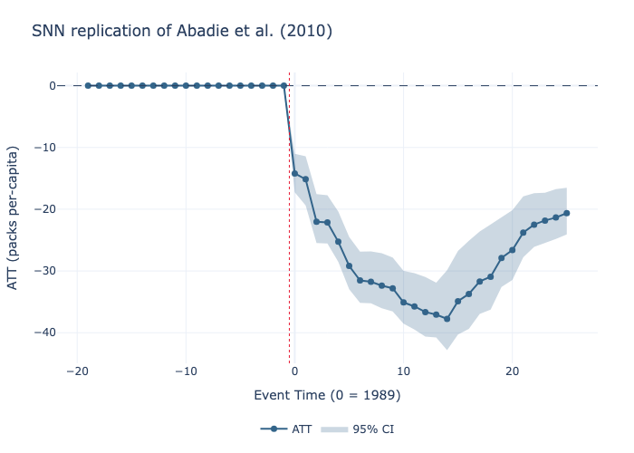
model.plot("gap")              # Average treatment effect on the treated (ATT) over time
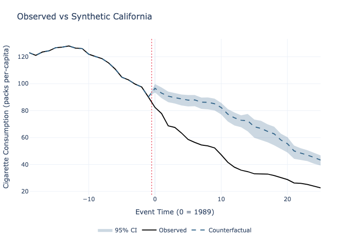
model.plot("counterfactual")   # Observed vs. counterfactual
Full Example — Replicating Abadie et al. (2010)
This example reproduces the well-known California tobacco control study.
Data: prop99.csv in the demos folder.
import pandas as pd
from synthnn import SNN

# 1. Load the data from Abadie et al. (2010)
df0 = pd.read_csv("prop99.csv", low_memory=False)

df = (
    df0
    .query("TopicDesc == 'The Tax Burden on Tobacco' "
           "and SubMeasureDesc == 'Cigarette Consumption (Pack Sales Per Capita)'")
    .loc[:, ["LocationDesc", "Year", "Data_Value"]]
    .rename(columns={
        "LocationDesc": "Unit",
        "Year":         "Time",
        "Data_Value":   "Y"
    })
)

# Drop territories & aggregate rows (keep 50 states)
bad_units = ["District of Columbia", "United States", "Guam",
             "Puerto Rico", "American Samoa", "Virgin Islands"]
df = df[~df["Unit"].isin(bad_units)]

# 2. Define the treatment indicator
df["W"] = ((df["Unit"] == "California") & (df["Time"] >= 1989)).astype(int)

# 3. Fit Synthetic-Nearest-Neighbors
model = SNN(
    unit_col="Unit",
    time_col="Time",
    outcome_col="Y",
    treat_col="W",
    variance_type="bootstrap",
    resamples=100,
    alpha=0.05
)

model.fit(df)

# 4. Inspect results
model.summary()

# 5. Plot the gap between treated and counterfactual
model.plot(
    title="SNN replication of Abadie et al. (2010)",
    xlabel="Event Time (0 = 1989)",
    ylabel="ATT (packs per-capita)"
).write_image("gap.png")

# 6. Plot observed vs counterfactual paths
model.plot(
    plot_type="counterfactual",
    title="Observed vs Synthetic California",
    xlabel="Event Time (0 = 1989)",
    ylabel="Cigarette Consumption (packs per-capita)"
).write_image("counterfactual.png")

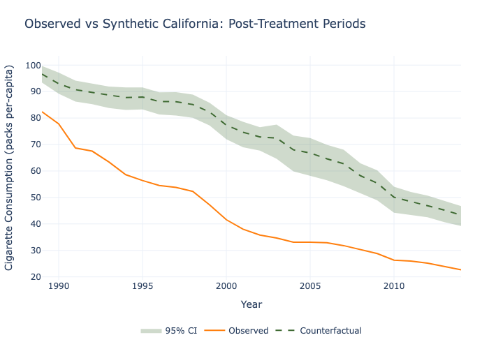
# 7. Same as before but with calendar time on the x-axis, only post-treatment periods, and custom colors
model.plot(
    plot_type="counterfactual",
    calendar_time=True,
    xrange=(1989, 2014),
    title="Observed vs Synthetic California: Post-Treatment Periods",
    xlabel="Year",
    ylabel="Cigarette Consumption (packs per-capita)",
    counterfactual_color="#406B34",  # green
    observed_color="#ff7f0e"         # orange
).write_image("graphics.png")

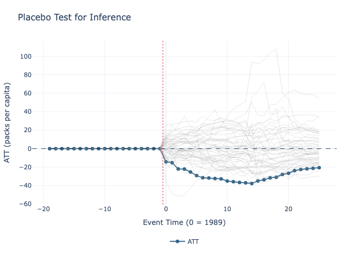
# 8. Inference using the placebo test (only works if there is exactly one treated unit)
model_pc = SNN(unit_col="Unit", time_col="Time", outcome_col="Y", treat_col="W",
               variance_type="placebo", alpha=0.05)
model_pc.fit(df)
model_pc.summary()

# 9. Plot the results, displaying the paths of the placebo treated units against the actual treated unit
model_pc.plot(show_placebos=True,
              title="Placebo Test for Inference",
              xlabel="Event Time (0 = 1989)",
              ylabel="ATT (packs per capita)").write_image("placebo.png")
Output
Click to expand
============================================================
SNN Estimation Results
============================================================

--- Overall ATT ---
estimate    method    se p_value ci_lower ci_upper
  -28.25 bootstrap 2.032       0   -32.07   -24.03


--- ATT by Event Time (Post-Treatment) ---

event_time    att N_units    se   p_value ci_lower ci_upper    method
         0  -14.2       1 1.651         0   -17.06   -11.28 bootstrap
         1 -15.15       1 2.077 3.015e-13   -18.75   -11.43 bootstrap
         2 -22.02       1 2.089         0   -26.16   -18.22 bootstrap
         3 -22.12       1 2.184         0   -26.15   -18.05 bootstrap
         4 -25.27       1 1.959         0   -28.55   -21.33 bootstrap
         5 -29.18       1 2.129         0   -32.97      -25 bootstrap
         6 -31.54       1 2.052         0   -35.08    -27.1 bootstrap
         7 -31.75       1 2.054         0    -35.6   -27.29 bootstrap
         8 -32.37       1 2.207         0    -36.2   -28.41 bootstrap
         9  -32.8       1 2.035         0   -36.08   -28.68 bootstrap
        10 -35.09       1 2.144         0   -38.64   -31.03 bootstrap
        11 -35.74       1 2.196         0   -39.74   -31.06 bootstrap
        12 -36.65       1 2.301         0   -41.26   -31.28 bootstrap
        13 -37.07       1 2.291         0    -41.5   -31.68 bootstrap
        14 -37.75       1 3.217         0   -44.07   -31.11 bootstrap
        15 -34.89       1 3.052         0   -40.54   -27.46 bootstrap
        16 -33.71       1 3.303         0   -39.55   -26.32 bootstrap
        17  -31.7       1 3.097         0   -37.31   -25.12 bootstrap
        18 -30.94       1 3.264         0    -36.9   -23.89 bootstrap
        19 -27.91       1 2.687         0   -32.99   -22.78 bootstrap
        20 -26.63       1 2.583         0   -31.33   -21.51 bootstrap
        21 -23.79       1 2.254         0   -27.74   -19.66 bootstrap
        22 -22.49       1 2.131         0   -26.36   -18.57 bootstrap
        23 -21.83       1 2.042         0   -25.58   -18.39 bootstrap
        24 -21.35       1 2.044         0   -24.94   -17.73 bootstrap
        25 -20.63       1 1.895         0   -24.19   -17.52 bootstrap

============================================================
============================================================
SNN Estimation Results
============================================================

--- Overall ATT ---
estimate placebo_p placebo_rank
  -28.25      0.08            4

Placebo Fisher p-value: 0.08  (rank 4/50)


--- ATT by Event Time (Post-Treatment) ---

 event_time    att N_units placebo_p
          0  -14.2       1       0.2
          1 -15.15       1      0.22
          2 -22.02       1      0.12
          3 -22.12       1      0.12
          4 -25.27       1      0.08
          5 -29.18       1      0.06
          6 -31.54       1      0.06
          7 -31.75       1      0.06
          8 -32.37       1      0.06
          9  -32.8       1      0.04
         10 -35.09       1      0.04
         11 -35.74       1      0.04
         12 -36.65       1      0.04
         13 -37.07       1      0.06
         14 -37.75       1       0.1
         15 -34.89       1      0.12
         16 -33.71       1       0.1
         17  -31.7       1      0.14
         18 -30.94       1      0.14
         19 -27.91       1      0.14
         20 -26.63       1       0.2
         21 -23.79       1       0.2
         22 -22.49       1      0.18
         23 -21.83       1      0.18
         24 -21.35       1      0.16
         25 -20.63       1      0.12

============================================================
Plots
Parameters
General
-
unit_col, time_col, outcome_col, treat_col (str) — Column names for unit ID, time, outcome, and treatment indicator.
-
variance_type (str) — Inference method:
"jackknife"— Leave-one-unit-out resampling"bootstrap"(default) — Block bootstrap on units"placebo"— Fisher randomization test (only when exactly one treated unit)
-
resamples (int) — Bootstrap resamples (default: 500)
-
alpha (float) — Significance level for confidence intervals (default: 0.05)
-
snn_params (dict) — Parameters for the
SyntheticNearestNeighborsimputer.
SNN Parameters (snn_params)
- n_neighbors (int) — Number of nearest neighbors (default: 1)
- weights (str) —
'uniform'or'distance' - random_splits (bool) — Use random splits in the algorithm
- max_rank (int) — Maximum rank for low-rank approximation
- spectral_t, linear_span_eps, subspace_eps (float) — Algorithm thresholds (default: 0.1)
- min_value, max_value (float) — Bounds for imputed values
- verbose (bool) — Print progress.
Plot Parameters
- plot_type —
"gap"or"counterfactual" - calendar_time (bool) — Use calendar time (for simultaneous adoption only)
- xrange (tuple) —
(min, max)for x-axis - title, xlabel, ylabel (str) — Labels
- figsize (tuple) —
(width, height) - color, observed_color, counterfactual_color, placebo_color (str) — Plot colors
- placebo_opacity (float) — Opacity for placebo lines (default: 0.25)
Output Attributes
After fitting, the model exposes:
- overall_att_ — Overall ATT with inference statistics
- att_by_event_time_ — ATT series by event time
- att_by_time_ — ATT series by calendar time
- individual_effects_ — Unit-level effects
- counterfactual_event_df_ — Observed vs. counterfactual (event time)
- counterfactual_df_ — Observed vs. counterfactual (calendar time)
Requirements
pandas,numpy,scipy,plotly,scikit-learn
Acknowledgments
The implementation in this package adapts and builds upon the code from the syntheticNN repository by Dennis Shen.
License
This project is licensed under the MIT License - see the LICENSE file for details.
Citation
If you use this package in your research, you can cite it as below.
@software{synthnn,
  author = {Lipkovitz, Rivka},
  month = jun,
  title = {{synthnn: a Python package for estimating treatment effects using Synthetic Nearest Neighbors}},
  url = {https://github.com/rivkalipko/synthnn},
  year = {2025}
}
Please also consider citing the authors of the original paper:
Agarwal, A., Dahleh, M., Shah, D., & Shen, D. (2023, July). Causal matrix completion. In The thirty sixth annual conference on learning theory (pp. 3821-3826). PMLR.
1 maintainer

Metadata
1 maintainer
Release files for synthnn 1.1.5
For a detailed explanation of source distributions (sdists) and built distributions (wheels), please see the package formats documentation.
Source distribution (sdist)
| File | Size | Uploaded | |
|---|---|---|---|
| synthnn-1.1.5.tar.gz | 27.0 kB | Details |
Built distribution (wheel)
| File | Interpreter | ABI | Platform | Reset |
|---|---|---|---|---|
| synthnn-1.1.5-py3-none-any.whl | Python 3 | none | any | Details |
Total release size: 50.4 kB
Release files / synthnn-1.1.5.tar.gz
| Download URL | synthnn-1.1.5.tar.gz |
|---|---|
| Size | 27.0 kB |
| Tags | Source |
|
SHA-256 checksum How to use checksums |
7961610f2a4db26b48732029fc051ab15b6b2d50b50a28a222fd77397cf02883
|
|
BLAKE2b-256 checksum How to use checksums |
d7d9813e199325751c5e83a24b2bfda8bc1250e7583065c70f411a08ab6ddd7a
|
| Upload date | |
|
Uploaded using Trusted Publishing? What is trusted publishing? |
No |
| Uploaded via |
twine/6.1.0 CPython/3.13.3
|
Release files / synthnn-1.1.5-py3-none-any.whl
| Download URL | synthnn-1.1.5-py3-none-any.whl |
|---|---|
| Size | 23.4 kB |
| Tags | Python 3 |
|
SHA-256 checksum How to use checksums |
4497a9f52d8416392c30bb86d393f11e53a7c95d978acfbd596c6d86c6c2574a
|
|
BLAKE2b-256 checksum How to use checksums |
014f394fd39395453c3df4d1b92507d263ad4d600b638275cece42ac2dfa5bd9
|
| Upload date | |
|
Uploaded using Trusted Publishing? What is trusted publishing? |
No |
| Uploaded via |
twine/6.1.0 CPython/3.13.3
|














