A Python package for estimating treatment effects using Synthetic Nearest Neighbors.

Project description
synthnn
A Python implementation of the Synthetic Nearest Neighbors (SNN) estimator for causal inference with panel data. The SNN estimator imputes each treated observation's untreated potential outcome using a synthetic nearest-neighbor "donor" pool, then averages the resulting effects to obtain the Average Treatment Effect on the Treated (ATT).
Features
- Flexible Panel Data Analysis: Supports both simultaneous and staggered treatment adoption
- Multiple Inference Methods: Jackknife, bootstrap, or Fisher-style placebo tests for uncertainty quantification
- Rich Visualization: Built-in plotting for gap plots and counterfactual comparisons
- Customizable Imputation: Configurable SNN parameters for different data characteristics
Installation
You can install synthnn from PyPI using pip:
pip install synthnn
Quick Start
import pandas as pd
from synthnn import SNN

# Load your panel data
df = pd.read_csv("your_panel_data.csv")

# Initialize the SNN model
model = SNN(
    unit_col="Unit",
    time_col="Time",
    outcome_col="Y",
    treat_col="W",
    variance_type="bootstrap",
    resamples=500,
    alpha=0.05
)

# Fit the model and get results
model.fit(df)
model.summary()

# Generate visualizations
model.plot("gap")  # ATT over time
model.plot("counterfactual")  # Observed vs counterfactual paths
Complete Example: Replicating Abadie et al. (2010)
This example demonstrates how to use SNN to replicate the famous California tobacco study. The prop99.csv file can be found in the demos folder of the GitHub repository.
import pandas as pd
from src.synthnn import SNN
# 1. Load the data from Abadie et al. (2010)
df0 = pd.read_csv("prop99.csv", low_memory=False)
df = (
df0
.query("TopicDesc == 'The Tax Burden on Tobacco' "
"and SubMeasureDesc == 'Cigarette Consumption (Pack Sales Per Capita)'")
.loc[:, ["LocationDesc", "Year", "Data_Value"]]
.rename(columns={
"LocationDesc": "Unit",
"Year": "Time",
"Data_Value": "Y"
})
)
# Drop territories & aggregate rows (keep 50 states + DC)
bad_units = ["District of Columbia", "United States", "Guam",
"Puerto Rico", "American Samoa", "Virgin Islands"]
df = df[~df["Unit"].isin(bad_units)]
# 2. Define the treatment indicator
df["W"] = ((df["Unit"] == "California") & (df["Time"] >= 1989)).astype(int)
# 3. Fit Synthetic-Nearest-Neighbors
model = SNN(
unit_col="Unit",
time_col="Time",
outcome_col="Y",
treat_col="W",
variance_type="bootstrap",
resamples=100,
alpha=0.05
)
model.fit(df)
# 4. Inspect results
model.summary()
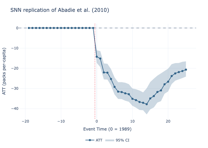
# 5. Plot the gap between treated and counterfactual
model.plot(
title="SNN replication of Abadie et al. (2010)",
xlabel="Event Time (0 = 1989)",
ylabel="ATT (packs per-capita)"
).write_image("gap.png")
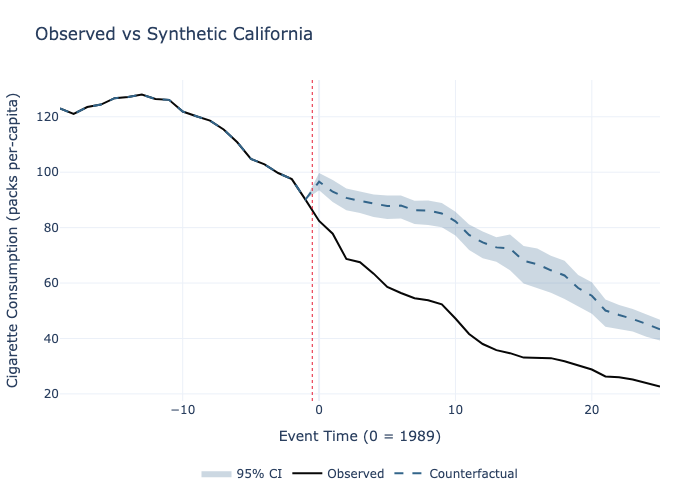
# 6. Plot observed vs counterfactual paths
model.plot(
plot_type="counterfactual",
title="Observed vs Synthetic California",
xlabel="Event Time (0 = 1989)",
ylabel="Cigarette Consumption (packs per-capita)"
).write_image("counterfactual.png")
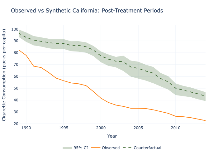
# 7. Same as before but with calendar time on the x-axis, only post-treatment periods, and custom colors
model.plot(
plot_type="counterfactual",
calendar_time=True,
xrange=(1989, 2014),
title="Observed vs Synthetic California: Post-Treatment Periods",
xlabel="Year",
ylabel="Cigarette Consumption (packs per-capita)",
counterfactual_color="#406B34", # green
observed_color="#ff7f0e" # orange
).write_image("graphics.png")
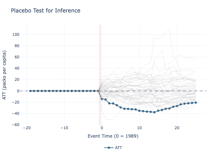
# 8. Inference using the placebo test (only works if there is exactly one treated unit)
model_pc = SNN(unit_col="Unit", time_col="Time", outcome_col="Y", treat_col="W",
variance_type="placebo", alpha=0.05)
model_pc.fit(df)
model_pc.summary()
# 9. Plot the results, displaying the paths of the placebo treated units against the actual treated unit
model_pc.plot(show_placebos=True,
title="Placebo Test for Inference",
xlabel="Event Time (0 = 1989)",
ylabel="ATT (packs per capita)").write_image("placebo.png")
Ouput
After running the above code, you will see the following output and graphs:
Click to expand SNN Estimation Results
============================================================
SNN Estimation Results
============================================================

--- Overall ATT ---
estimate    method    se p_value ci_lower ci_upper
  -28.25 bootstrap 1.962       0   -32.04   -24.98


--- ATT by Event Time (Post-Treatment) ---

event_time    att N_units    se   p_value ci_lower ci_upper    method
         0  -14.2       1 1.596         0   -17.33   -11.36 bootstrap
         1 -15.15       1 2.179 3.554e-12   -20.21   -11.35 bootstrap
         2 -22.02       1 2.327         0   -26.86    -17.3 bootstrap
         3 -22.12       1 2.399         0   -27.04   -17.62 bootstrap
         4 -25.27       1 2.254         0   -29.65   -20.97 bootstrap
         5 -29.18       1 2.282         0   -33.35   -25.59 bootstrap
         6 -31.54       1 2.109         0   -35.63   -28.13 bootstrap
         7 -31.75       1 2.102         0   -36.12   -28.25 bootstrap
         8 -32.37       1 2.161         0   -36.45   -28.93 bootstrap
         9  -32.8       1 1.968         0   -36.76   -29.28 bootstrap
        10 -35.09       1 1.985         0   -39.17   -32.11 bootstrap
        11 -35.74       1 2.094         0      -40   -32.39 bootstrap
        12 -36.65       1 2.113         0   -41.03    -33.1 bootstrap
        13 -37.07       1 2.212         0   -41.73   -33.17 bootstrap
        14 -37.75       1 2.963         0   -43.81   -33.19 bootstrap
        15 -34.89       1 3.064         0   -41.52   -30.25 bootstrap
        16 -33.71       1 3.316         0   -40.94   -28.79 bootstrap
        17  -31.7       1 3.056         0   -38.04   -26.56 bootstrap
        18 -30.94       1 3.241         0   -37.83   -25.61 bootstrap
        19 -27.91       1 2.744         0   -33.42   -23.05 bootstrap
        20 -26.63       1 2.675         0   -31.88   -22.27 bootstrap
        21 -23.79       1 2.277         0   -28.14    -19.5 bootstrap
        22 -22.49       1 2.156         0    -26.7   -18.41 bootstrap
        23 -21.83       1 2.102         0   -26.03   -18.08 bootstrap
        24 -21.35       1 2.077         0   -25.09   -17.35 bootstrap
        25 -20.63       1 1.961         0   -24.23   -17.15 bootstrap

============================================================
============================================================
SNN Estimation Results
============================================================

--- Overall ATT ---
estimate placebo_p placebo_rank
  -28.25      0.08            4

Placebo Fisher p-value: 0.08  (rank 4/50)


--- ATT by Event Time (Post-Treatment) ---

 event_time    att N_units placebo_p
          0  -14.2       1       0.2
          1 -15.15       1      0.22
          2 -22.02       1      0.12
          3 -22.12       1      0.12
          4 -25.27       1      0.08
          5 -29.18       1      0.06
          6 -31.54       1      0.06
          7 -31.75       1      0.06
          8 -32.37       1      0.06
          9  -32.8       1      0.04
         10 -35.09       1      0.04
         11 -35.74       1      0.04
         12 -36.65       1      0.04
         13 -37.07       1      0.06
         14 -37.75       1       0.1
         15 -34.89       1      0.12
         16 -33.71       1       0.1
         17  -31.7       1      0.14
         18 -30.94       1      0.14
         19 -27.91       1      0.14
         20 -26.63       1       0.2
         21 -23.79       1       0.2
         22 -22.49       1      0.18
         23 -21.83       1      0.18
         24 -21.35       1      0.16
         25 -20.63       1      0.12

============================================================
Parameters
General Parameters
- unit_col, time_col, outcome_col, treat_col (str): Column names for unit ID, time, outcome, and treatment indicator
- variance_type (str): Method for uncertainty quantification:
"jackknife": Leave-one-unit-out resampling"bootstrap": Block bootstrap on units (default)"placebo": Fisher randomization test for when there is exactly one treated unit
- resamples (int): Number of bootstrap resamples (default: 500)
- alpha (float): Significance level for confidence intervals (default: 0.05)
- snn_params (dict): Parameters for the underlying SyntheticNearestNeighbors imputer
SNN Parameters
The snn_params dictionary can include:
- n_neighbors (int): Number of nearest neighbors to use (default: 1)
- weights (str): Weight function for neighbors (
'uniform'or'distance') - random_splits (bool): Whether to use random splits in the algorithm
- max_rank (int): Maximum rank for low-rank approximations
- spectral_t (float): Spectral threshold parameter (default: 0.1)
- linear_span_eps (float): Linear span epsilon (default: 0.1)
- subspace_eps (float): Subspace epsilon (default: 0.1)
- min_value, max_value (float): Bounds for imputed values
- verbose (bool): Whether to print progress information
Plot Parameters
- plot_type (str):
"gap"for ATT series or"counterfactual"for observed vs counterfactual paths - calendar_time (bool): Use calendar time instead of event time (simultaneous adoption only)
- xrange (tuple): Range for x-axis as
(min, max) - title, xlabel, ylabel (str): Custom labels
- figsize (tuple): Figure size as
(width, height) - color, observed_color, counterfactual_color (str): Custom colors for different plot elements
Output
After fitting, the model provides several key attributes:
- overall_att_: Overall average treatment effect with inference statistics
- att_by_event_time_: ATT series by event time with confidence intervals
- att_by_time_: ATT series by calendar time
- individual_effects_: Unit-level treatment effects
- counterfactual_event_df_: Observed vs counterfactual paths by event time
- counterfactual_df_: Observed vs counterfactual paths by calendar time
Requirements
pandasnumpyscipyplotlykaleidofor exporting images- The
SyntheticNearestNeighborsbase class (included in package)
Acknowledgments
The implementation in this package adapts and builds upon the code from the syntheticNN repository by Dennis Shen.
License
This project is licensed under the MIT License - see the LICENSE file for details.
Citation
If you use this package in your research, you can cite it as below.
@software{synthnn,
  author = {Lipkovitz, Rivka},
  month = jun,
  title = {{synthnn: a Python package for estimating treatment effects using Synthetic Nearest Neighbors}},
  url = {[https://github.com/rivkalipko/synthnn](https://github.com/rivkalipko/synthnn)},
  year = {2025}
}
Please also consider citing the authors of the original paper:
Agarwal, A., Dahleh, M., Shah, D., & Shen, D. (2023, July). Causal matrix completion. In The thirty sixth annual conference on learning theory (pp. 3821-3826). PMLR.


Download files
Download the file for your platform. If you're not sure which to choose, learn more about installing packages.
Source Distribution
Built Distribution
Filter files by name, interpreter, ABI, and platform.
If you're not sure about the file name format, learn more about wheel file names.
Copy a direct link to the current filters
File details
Details for the file synthnn-1.1.2.tar.gz.
File metadata
- Download URL: synthnn-1.1.2.tar.gz
- Upload date:
- Size: 27.8 kB
- Tags: Source
- Uploaded using Trusted Publishing? No
- Uploaded via: twine/6.1.0 CPython/3.13.3
File hashes
| Algorithm | Hash digest | |
|---|---|---|
| SHA256 |
6cba56711cfc6f56c69f2fc3838d782061ca9de6e5ba66cc1c8e076be39e0520
|
|
| MD5 |
f3d04ff183573a85bc377a811d5fe961
|
|
| BLAKE2b-256 |
a40275286e23a3f29aa21abd2ba69396d7bb181c6604b5b1679b0aba0232e332
|
File details
Details for the file synthnn-1.1.2-py3-none-any.whl.
File metadata
- Download URL: synthnn-1.1.2-py3-none-any.whl
- Upload date:
- Size: 24.0 kB
- Tags: Python 3
- Uploaded using Trusted Publishing? No
- Uploaded via: twine/6.1.0 CPython/3.13.3
File hashes
| Algorithm | Hash digest | |
|---|---|---|
| SHA256 |
3d8c0038d16476c8503fb9e3c0539512d0a24f2a2cecfc1dd6766fee65ebe068
|
|
| MD5 |
7b0444608512d4211cbe7231b31687c3
|
|
| BLAKE2b-256 |
96f8005e30c2e0a7edcd48a8b57e6a484ef8a6b3c2f26a257119fe3d7c849afa
|


