
🌊 ZimaBlue
Where robotic pool cleaners come to play.
Build pools, test controllers, measure cleaning, and replay every run.







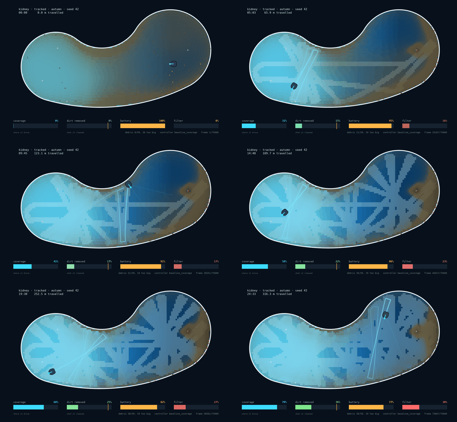
25 simulated minutes in a kidney pool, replayed at 260×.
Watch the coverage and dirt meters drift apart.
Give ZimaBlue a pool, a cleaner, some dirt and a control algorithm. It simulates the run, records it, replays it, and scores how clean the pool actually got. Coverage records how much floor the robot drove over; cleanliness records the dirt it removed. The two numbers often diverge.
git clone https://github.com/JGalego/ZimaBlue
cd ZimaBlue
pip install -e ".[dev]"
zimablue demo
The install needs no GPU, ROS, Docker, Omniverse or multi-gigabyte assets.

A real run, from command to metrics to a replayable .zbr recording.
What's in it
| 🏊 | Pools | Presets from a plain rectangle to a kidney and a Bunimovich stadium, or your own Shapely outline with a pluggable depth model. Drains, skimmers, stairs and obstacles come out of the navigable area. |
| 📷 | Pools from photographs | Trace one image, or fuse several perspective-corrected phone views with cross-view agreement and measured depth. Colour rules by default, or SAM if you have a checkpoint. |
| ✏️ | Pools from drawings | Sketch one on a napkin or in a paint program and trace it. Copes with a lifted pen, notes scribbled inside the outline, and the shadow across a photo of paper. |
| 🤖 | Cleaners | Composed from chassis, drive, cleaning head and power. A custom robot needs no changes to ZimaBlue. |
| 🎨 | Cleaner designs | Silhouettes with real differences, so a domed suction unit does not look like a quad-brush commercial machine. Drawing only — the physics is the chassis. |
| 📡 | Sensors that lie | Encoders, IMU, pressure, bump switches, sonar, a turbidity probe, all through one noise, bias, latency, dropout and saturation pipeline. Faults on a schedule. |
| 🍂 | Dirt that behaves | Density, grain size, adhesion and pickup difficulty, settling by Ferguson & Church rather than Stokes. Fine dirt rides the return jets, what floats drifts to the skimmer, and the robot's own wake stirs up what it drives over. Scenarios from clean to neglected_pool, and pool_party, where dirt keeps arriving and swimmers keep stirring it — clean becomes a rate you hold, not a state you reach. |
| 🧭 | Controllers | Boustrophedon coverage, random bounce, an EKF-and-occupancy-map planner, and ground-truth oracles to bound the problem. |
| 🗺️ | Coverage path planning | Offline decompositions and online rules from the classical literature, Spiral-STC through a spectral ergodic controller. See planners. |
| 🧗 | Walls and the waterline | The wall is an area, not a line: a floor robot brushes the cove and nothing above it, a grip-capable one climbs to the waterline, and both are scored against the wall's real square metres. |
| 🛥️ | Fleets | Several cleaners in one pool, sharing the dirt and getting in each other's way. Mix robot designs and controllers, divide the pool between them, or coordinate without dividing it. See fleets. |
| ⚖️ | Scored on what actually differs | Coverage, overlap, turning, the worst gap left behind, anytime behaviour, energy. No single winner, and a matrix plot that shows why. |
| 📊 | Metrics that disagree | Coverage and cleanliness scored separately, each with a spatial companion. The whole point is that they rank controllers differently. |
| 🎬 | Watch it | Top down, chase cam, the dirt cam from the robot's own bumper, and a 3D basin. GIF, MP4 or an interactive window. |
| 💾 | Reproducible recordings | The .zbr format: same version, platform, scenario and seed gives a bit-identical run. Rerun one with a different policy using counterfactual replay. |
| 🪞 | Digital twins | Calibrate bounded model parameters against measured trajectories, then run a read-only live shadow beside hardware and monitor sensor residuals. |
| 🧪 | Experiments | YAML scenarios, batch sweeps, adaptive replicated experiments, and frozen benchmark regression gates. |
| ∂ | Motion gradients | Exact free-space differential-drive integration with analytical state, command and track-width Jacobians for MPC and sensitivity analysis. See differentiable physics. |
| 🕹️ | A Gymnasium environment | Train a policy against the same simulator, then run it as an ordinary controller so it is scored like every other one. |
| 🔌 | Runs on real hardware | The control loop with no simulator underneath: sensor adapters, a wheel-speed loop, a watchdog. Writes the same .zbr. See on a robot. |
| 📈 | Checked against a real robot | The pose estimator scored against a Pioneer 3-DX's logged trajectory, not only against motion we generated ourselves. |
| 🌀 | Dynamical-systems analysis | Poincaré sections, transfer operators, the ergodic metric, Lyapunov divergence. Finds where a controller gets stuck rather than scoring it. See behaviour. |
Contents
- Build a pool
- Add a cleaner — make it look like yours
- Make it dirty
- Run it
- Plan it
- Send a fleet
- Watch it — from behind, from the bumper, in 3D
- Measure it
- Check it against a real robot
- Analyse it
- Scale it
- Extend it
- Read more
- Did you know?
Build a pool
import zimablue as zb

pool = zb.make_pool("kidney")  # rectangular · sloped · l_shaped · oval · stairs
# stadium · mushroom  (chosen for their dynamics)
Geometry is a Shapely polygon plus a pluggable depth model, so a sloped floor and a flat one differ only in which model they hold. Drains, returns, skimmers, stairs and obstacles hang off it; the blocking ones come out of the navigable area, so coverage is measured against the floor the robot can actually reach.
The kidney is a chain of four circular arcs — two lobes, a belly under
both, a scoop bitten out between them — meeting where their circles are
tangent, which is how a kidney is set out on site. So it has no corners, and a
wall follower meeting a corner behaves differently from one tracing a curve.
Every radius is an argument: zb.make_pool("kidney", length=16.0, scoop_radius=2.0) gives a bigger pool with a deeper bite.
Have a photo instead of a spec? zb.pool_from_image("backyard.jpg", sample=(640, 410), width=8.4) finds the water, traces its edge and scales it.
A photograph carries no scale of its own, so one real measurement is required;
for a shot taken from the poolside, four points on a rectangle you can measure
also undo the perspective, which is worth about 27% of the area. See
imaging.
Colour rules find the water by default. Point segmenter=SamSegmenter.load(...)
at a SAM export and a model finds it instead — worth it for a black-bottomed
pool, or one half in shade. On a drone photo the two agree to 3.7%, which is a
reasonable amount of confidence in both. See machine learning.
In a notebook, zb.preview(pool) renders it in the browser — drag to rotate,
scroll to zoom. The pool's geometry is shipped to the page as JSON and
projected there, so it needs no widget extensions and keeps working in an
exported HTML file. Hand it a finished run and it tints the floor with the
dirt left behind and draws the path that was driven.
Add a cleaner
Cleaners are built from components:
robot = zb.Cleaner(
    chassis=zb.Chassis(length=0.45, mass=10.5),
    cleaning=zb.CleaningSystem(
        brush=zb.Brush(width=0.38, aggressiveness=1.2),
        filter=zb.Filter(capacity=1200.0, mesh=45e-6),
    ),
    sensors=[zb.Encoder(), zb.IMU(), zb.Sonar(beam_angles=(0.0, 0.7, -0.7))],
)
Encoders, IMU, pressure/depth, contact, sonar and a turbidity probe share one pipeline of sampling rate, noise, bias with random walk, latency, quantisation, saturation, dropout and stuck values. Encoders report wheel speed, so odometry drifts because the wheels really do slip; no error is injected to make it happen. The turbidity probe is the intake's "dirt detect": it reads the dirt density under the hull plus the water's own haze, which is the one signal that lets a deployable controller chase grams instead of area.
You can break a sensor on purpose:
robot.sensors.sonar.inject_fault(
    bias=0.15,  # reads 15 cm long
    dropout_probability=0.02,  # loses 2% of pings
    start_time=300.0,  # ...starting five minutes in
)
Make it look like yours
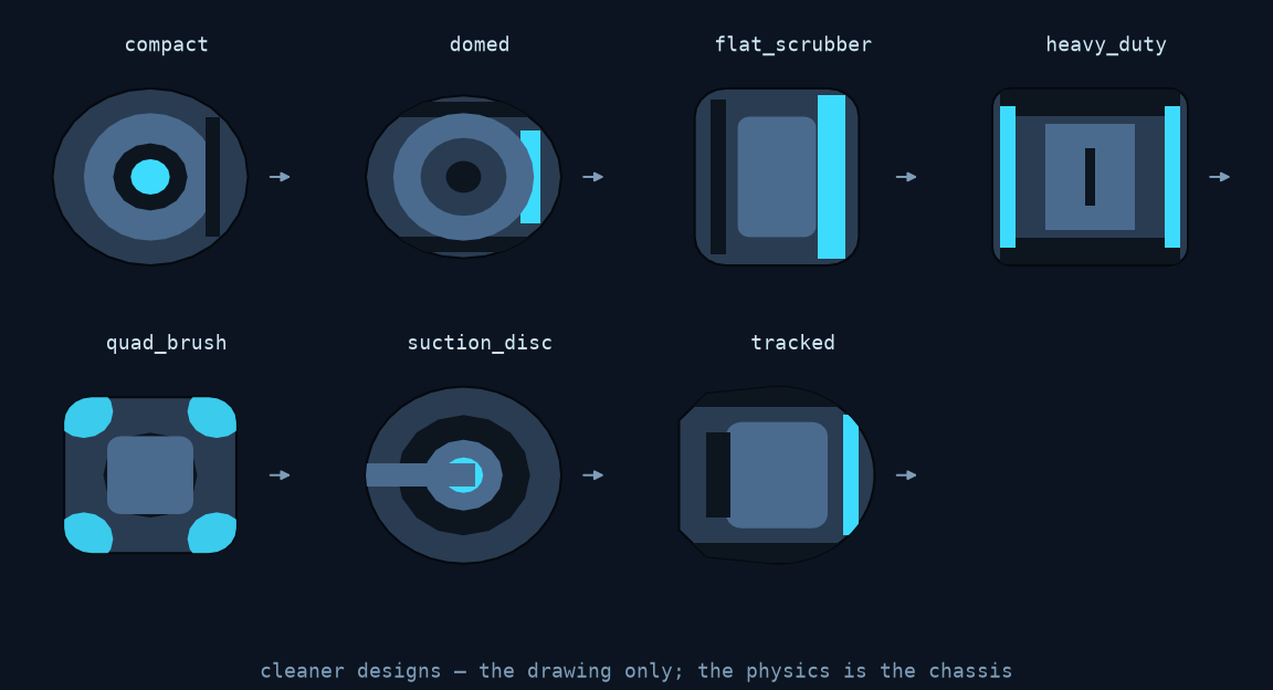
robot = zb.make_robot("tracked")
robot.design = zb.make_design("quad_brush")
Each archetype is named by form rather than by product, because the form is the useful abstraction and a library has no business shipping traced outlines of somebody's industrial design. To match a specific machine, measure it:
from zimablue.robot import CleanerDesign, Part
from zimablue.robot.design import ellipse, bar

mine = zb.Cleaner(
    name="mine",
    design=CleanerDesign(
        name="mine",
        body=ellipse(0.5, 0.44),
        parts=(Part(bar(0.34, 0.30, 0.09), colour="#3ddcff", lift=0.05, name="brush"),),
    ),
)
Coordinates run −0.5 to 0.5 and are scaled by the chassis, so any design fits any robot. It is a drawing and nothing else. Collision uses the chassis rectangle, cleaning uses the swath width, traction uses the mass — swapping a design changes every rendered pixel and not one number in the metrics. A drawing that quietly moved the results would be the worst kind of bug, so there is a test that a run scores identically whichever design it wears.
Make it dirty
Dirt carries density, particle size, adhesion and a settling velocity derived from the Ferguson–Church equation — 350 µm sand comes out at 47.6 mm/s against a measured ~45. Sediment and algae live in continuous rasters; leaves and twigs are discrete items, some too big for the intake to swallow.
Removal is gated by how much agitation breaks the bond, so the brush matters more the more adhered the dirt is: ~1.0× for sand, 2.2× for algae, 3.5× for biofilm. Turn the brush off and a robot can drive over algae all day.
Run it
sim = zb.Simulation(pool="kidney", robot="tracked", dirt="autumn", seed=42)
result = sim.run(minutes=30)

print(result.metrics.summary())
result.save("runs/example.zbr")
  coverage            83.0 %   (walls 77 %)
  dirt removed        39.2 %   (385 g of 982 g)
  uniformity          66.7 %
  revisits            1.94   extra passes/cell
  distance           389.1 m
  runtime             30.0 min
  energy              33.3 Wh   (battery 72 % left)
  collisions           513
  stuck                  0 events, 0.0 s
  debris                39 collected of 59, 20 too big for the intake
  dirt ceiling        91.8 %   (80 g this intake cannot lift)
  termination       duration
Driving it is a boustrophedon baseline, a random-bounce floor, a map-building
systematic controller, or the ground-truth oracles, which are explicitly
not deployable: lawnmower_oracle drives a perfect path, dirt_oracle
heads for whatever is dirtiest. Yours needs a class with reset and step,
and sees sensor readings only.
Or train one. zimablue[rl] registers the same simulation as the ordinary
Gymnasium environment ZimaBlue-v0. An observation is the robot's sensor
readings, an action is its two track speeds, and the default reward is dirt
collected. The loop runs at 24× real time on one CPU core with no GPU.

This is training, not playback. Each cyan point is a policy tried in the live pool on the left; the yellow line is the best found so far. The dashed line is not a hoped-for score: it is the known constant-curvature optimum.
Watch the same run update in a window on your machine:
pip install "zimablue[rl,viz]"
python examples/live_training.py
The pool floor is a constant-width loop around an island. Its shortest
non-overlapping coverage path is the centreline, and differential-drive
kinematics gives the exact track speeds for that circle. Cross-entropy policy
search starts from random track speeds and discovers the stable orbit: with
the fixed demo seed, its score jumps in generation three and reaches 99% of
the reference in generation four. For a full PPO run on an ordinary pool, use
python examples/train_policy.py.
Here is a complete first episode. The action is simply the left and right track speed from -1 (full reverse) to 1 (full forward):
import gymnasium as gym
import numpy as np
import zimablue.rl  # registers ZimaBlue-v0

env = gym.make(
    "ZimaBlue-v0",
    pool="rectangular",
    dirt="light_sediment",
    minutes=1,
    render_mode="rgb_array",
)
observation, info = env.reset(seed=42)

finished = False
total_reward = 0.0
while not finished:
    action = np.array([1.0, 0.72])  # left track, right track
    observation, reward, terminated, truncated, info = env.step(action)
    total_reward += reward
    finished = terminated or truncated

print(f"reward: {total_reward:.1f}")
print(f"coverage: {info['coverage']:.1%}")
print(f"dirt removed: {info['dirt_removed']:.1%}")
env.close()
Install it with pip install "zimablue[rl]". Replace the one action = ...
line with a model prediction to start training; the rest is standard
Gymnasium. Reward design matters: pay for coverage and a policy can learn to
drive beautifully over dirt it never picks up. See machine learning.
systematic runs an EKF over position, heading and gyro bias. The bias is
only observable when the robot stops — a stationary gyro's reading is its
bias — so zero-velocity updates are what keep heading from fanning out over
half an hour.
Run the same version on the same platform, with the same scenario and seed,
and you get the exact same recording every time. That comes from a fixed
timestep, no wall-clock reads while stepping, and one seeded RNG tree whose
named streams mean adding a sensor never shifts another's noise. .zbr is a
ZIP of a JSON manifest, columnar npz frames, sparse events and dirt
keyframes — unzip it and read it with numpy.load. Pool geometry and robot
config are embedded, so a recording stays replayable after the preset it came
from changes.
Plan it
zimablue.planners covers most of the single-robot coverage literature.
The offline planners are given the pool and compute a whole route; the
online ones decide the next move from what the sensors just said.
from zimablue.planners import PathFollower

zb.Simulation(pool="kidney", controller="bsa").run(minutes=20)

morse = PathFollower("morse")
zb.Simulation(pool="kidney", controller=morse, expose_truth=True).run(minutes=20)
The online ones share everything except the decision. One base class owns the EKF, the occupancy grid, the bump recovery and the driving; each algorithm implements one method that returns the next cell. If they each had their own motion layer, a difference in coverage could always be the motion layer's fault.
Following a plan is not free, and PathFollower is where the bill arrives.
Drive it from the true pose and you have measured the route; drive it from
dead reckoning and you have measured the route plus the localisation. On the
rectangular pool sweep_optimal reaches 70.5% on truth and 49.6% on odometry
— twenty-one points of the plan's value never reaches the floor.
python examples/compare_planners.py --minutes 20 --jobs 4 --plots out/
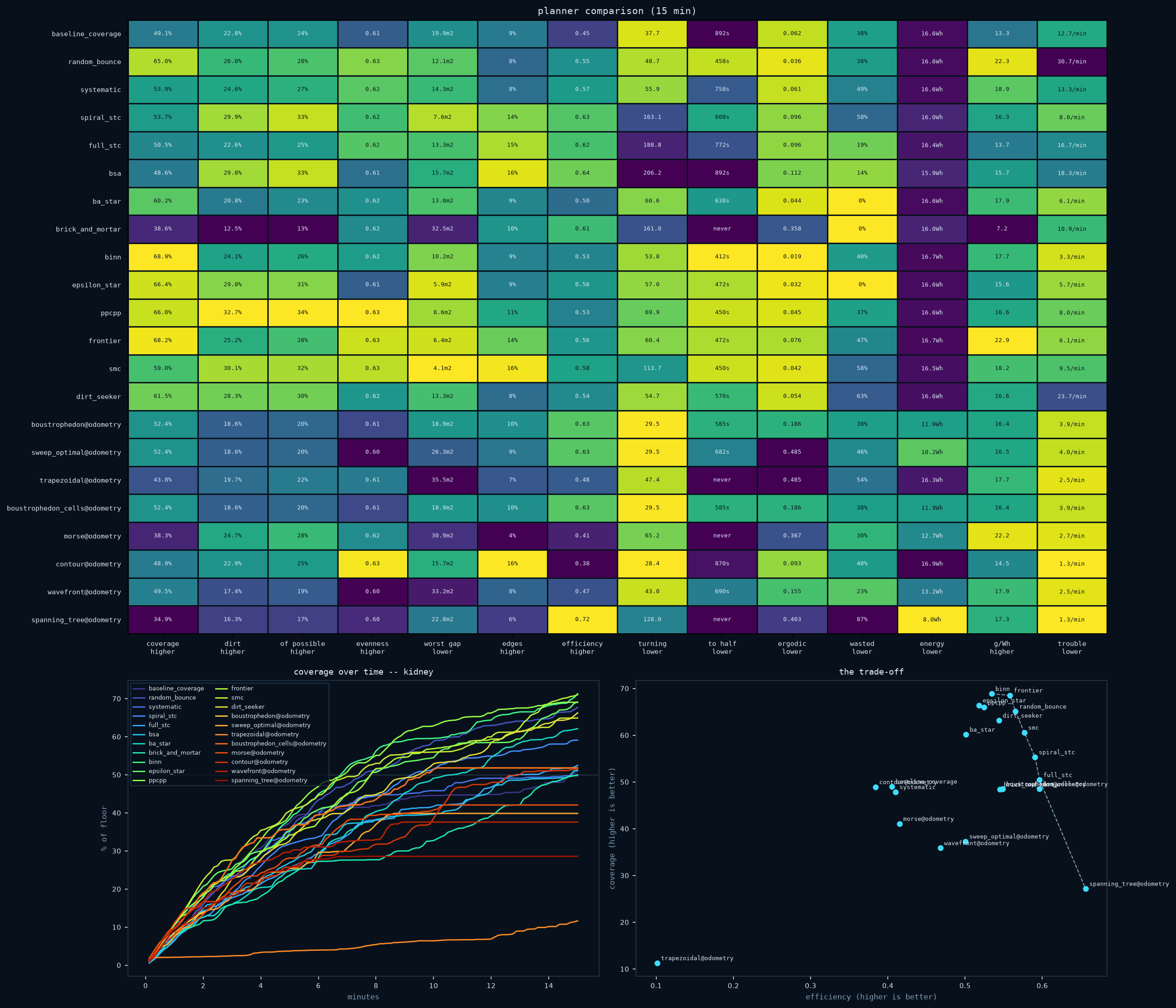
Each planner is measured on coverage, dirt, evenness, worst gap, edges, path efficiency, turning per metre, time to half the pool, ergodic error, wasted time, energy and collisions — deliberately not collapsed into one number. The columns that earn their place are efficiency, turning and the worst gap: a planner can reach 95% by driving over everything three times, and 90% coverage means something different depending on whether it left a thin margin everywhere or a whole corner.
The headline is not the winner. It is that random_bounce — drive straight,
turn at random when you hit something — beats most of the table, including
planners with completeness proofs. Coverage path planning
has the full table, and an animated mosaic of every planner cleaning the
kidney at once.
Send a fleet
result = zb.Fleet(pool="kidney", robots=3, controllers="auction").run(minutes=20)
print(result.summary())
  robots            3
  team coverage       90.7 %
  overlap             83.7 %   (floor two or more robots both did)
  speedup             1.25 x   (against the best single member)
  balance             0.85     (shortest run / longest)
  encounters           136     (robot-on-robot)
Coverage is the least interesting number there. Speedup has a ceiling equal to the robot count, and how far short it falls is the cost of sharing a pool. Overlap is the floor more than one robot did. Balance catches the failure coverage hides completely: one robot working while another parks in a corner it was assigned.
The robots share one dirt field, collide with each other, and see each other on the sonar. What they know about each other went over a radio, as estimates — so a fleet inherits every member's localisation error and then has to coordinate through it.
Either cut the pool up and hand each piece to a single-robot planner
(voronoi, geodesic, strips, darp, forest), or coordinate without
cutting anything (mstc, auction, binn_swarm, smc_swarm, and the
shared-map version of every online planner, which is the default).
from zimablue.planners import partitioned

zb.Fleet(pool="kidney", robots=3, controllers=partitioned("darp", "sweep_optimal"))
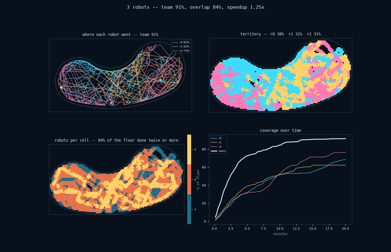
The result worth the trouble: the same DARP partition followed from the true pose gives a 2.92x speedup with 0.3% overlap — near-perfect division of labour — and followed on dead reckoning gives 2.05x with 34%. The partition survives in the plan and evaporates in the execution.
And on a kidney pool the fourth robot is where the team stops being a team: coverage keeps climbing, 43% → 64% → 78% → 84%, while speedup peaks at three robots and then falls. Half the pool is already being done twice at three, and the fourth buys six points of floor for eight more of overlap and half again as many collisions. See fleets.
Watch it
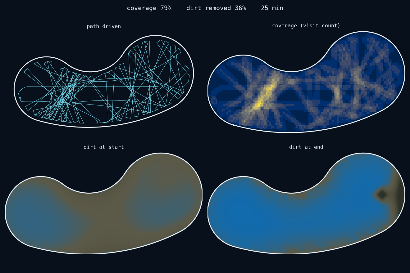
zimablue replay runs/example.zbr
Playback runs at 0.25× to 25×, with pause, scrub, step and speed control; 1× plays the run at the speed it happened. The cleaned swath is drawn under the dirt, so a patch the robot drove over but failed to clean still looks dirty. Sonar beams, wall contacts, battery and filter fill are all on screen, and if the controller publishes a pose estimate it appears as an amber ghost drifting away from the true position.
Headless? zimablue replay run.zbr --gif out.gif.
From behind
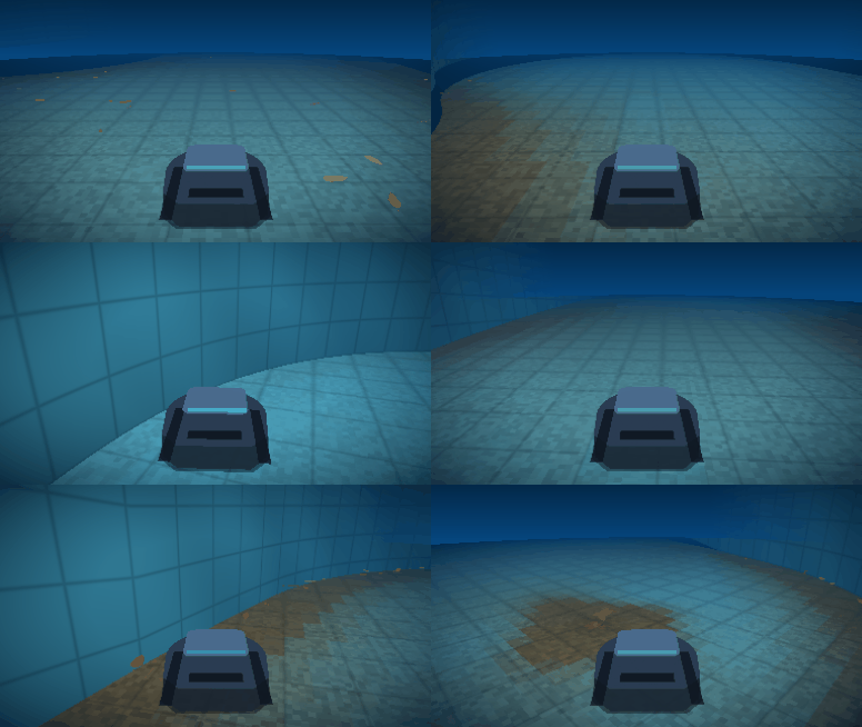
Chase cam. Close enough to see the brushes, far enough to see the swath.
Same two minutes: near enough in time to watch the dirt line recede.
zimablue replay runs/example.zbr --chase --gif out.gif
The other two views each hide something. From above the robot is a postage stamp, so you read the path and lose the machine. From the bumper you never see the machine at all. A metre back and half a metre up you get both, and because the robot is now in front of the camera it has to be drawn — from its own design, so a domed suction unit and a quad-brush commercial machine look like different machines.
The camera follows with lag. Bolt it rigidly and a turn reads as the pool rotating, which is disorienting and wrong; let its heading chase the robot's and the turn reads as the robot swinging across frame.
From the bumper
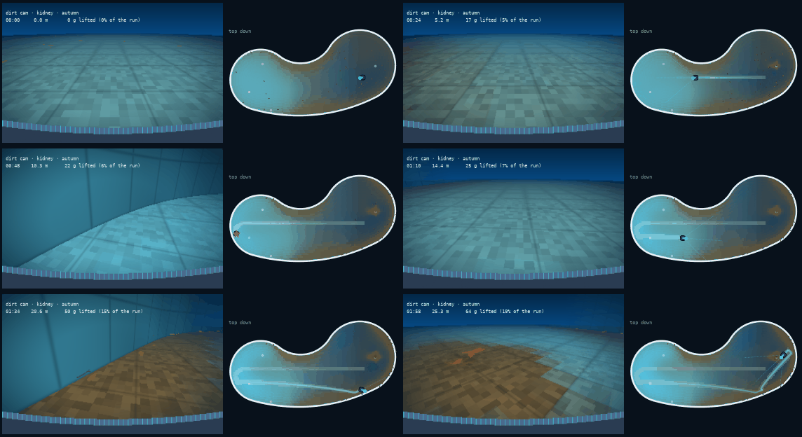
Dirt cam, with the top-down view alongside — the first two minutes, at two
simulated seconds a frame. The two panels disagree constantly.
zimablue replay runs/example.zbr --dirtcam --gif out.gif
Watching from above is calming. From 18 cm off the floor the same pool is a silt plain with leaves in it, which is closer to what a cleaner is driving through. From above you see where the robot went; from down here you see what it left behind.
It uses inverse perspective mapping over the same dirt raster the metrics are computed from. Those rays also meet depth-aware panels along the exact pool curve, so the tiled wall rises from the floor without needing a 3D engine.
In 3D
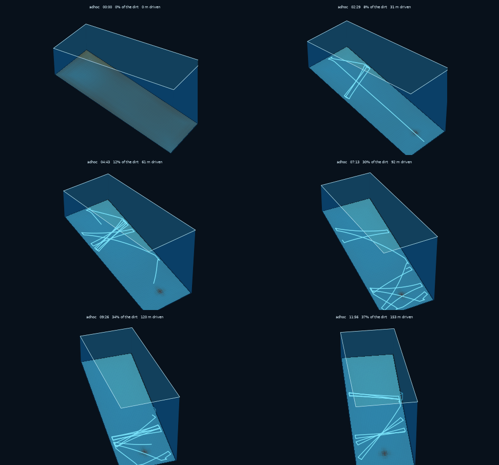
A sloped pool: 1.0 m at the shallow end, 2.4 m at the deep end.
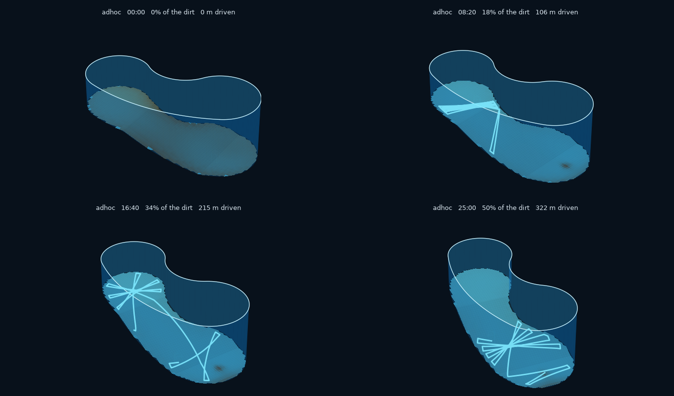
zimablue replay runs/example.zbr --3d --gif out.gif
The floor is a surface built from the pool's depth model, the walls are extruded from its boundary, and the robot sits at the local floor depth — so in a sloped pool it really is metres lower at the deep end. The camera orbits slowly for parallax, and vertical scale is exaggerated about 3.6× because a 12 m pool 2 m deep is otherwise a pancake.
This renders in 3D; it does not simulate in 3D. The motion still comes from the 2D backend. A 3D backend — buoyancy, contact, wall climbing, cameras — is designed but not built, and the roadmap says so.
Measure it
Coverage is where the robot drove. Cleanliness is what it removed. They come apart, and most simulators will not tell you so.
The oracle makes it obvious. Over 30 minutes in a kidney pool:
| controller | coverage | dirt removed | distance |
|---|---|---|---|
lawnmower_oracle (ground truth) |
88.5% | 33.1% | 181 m |
random_bounce |
84.3% | 49.5% | 382 m |
baseline_coverage |
83.0% | 39.2% | 389 m |
The ranking inverts. Best coverage is worst cleaning: the oracle drives a perfect path, finishes early and stops, while the scrappier controllers keep going over the same adhered dirt, which is what actually removes it — twice as much driving for sixteen more points of dirt. Report only coverage and you rank these three exactly backwards.
Better localisation currently makes things worse. Calibrating the odometry improves the mapping controller's position estimate fivefold and halves its coverage.
encoder_scale |
position error | coverage |
|---|---|---|
| 1.00 (uncalibrated) | 13.7 m | 73.9% |
| 0.94 (calibrated) | 3.8 m | 52.6% |
The estimator is not at fault — 3.8 m after 340 m of travel with no absolute reference is respectable dead reckoning. The planner is. With a poor estimate the lane plan is effectively randomised and the robot wanders widely, covering ground the way random bounce does; with a good one it runs short disciplined lanes and spends its time turning. Coverage is being won by accident, and fixing that is the top roadmap item.
Check it against a real robot
Those numbers all come from motion this package generated, judged against ground truth it also generated. That is unfalsifiable, so there is now a path that is not.
python tools/fetch_trajectory.py --all
python examples/replay_real_trajectory.py
A Pioneer 3-DX driving a real building, tracked at 300 Hz by a real motion capture rig. The shipped sensor models are driven from that motion and the estimator is scored against where the robot actually was:
| log | drove | final error | mean | worst |
|---|---|---|---|---|
pioneer_360 |
17.0 m | 0.18 m | 0.22 m | 0.44 m |
pioneer_slam |
42.5 m | 0.15 m | 0.34 m | 1.08 m |
pioneer_slam2 |
23.3 m | 2.16 m | 0.86 m | 2.17 m |
The motion is real, including a full second where the tracker lost the robot.
The sensors are not — the noise is still ours — and there is no slip, so the
estimator is being flattered in a known direction. Even so it says something
the table above could not: the 13.7 m of drift is the slip model's doing, not
a real trajectory being hard to integrate. And pioneer_slam2 ends 39° out on
heading because the gyro bias is only observable when the robot stops, and
that one rarely does.
The whole control loop runs on real hardware too, through the same
ControlInput and DriveCommand a controller already sees. See
on a robot.
Analyse it
Coverage and cleanliness say what a run achieved. They say nothing about how the robot behaved — whether it repeated itself, how fast it forgot where it started, whether the room was doing the work.
from zimablue.dynamics import transfer_operator, ergodic_score

operator = transfer_operator([run_a, run_b, run_c])
print(operator.summary())  # mixing rate
labels = operator.almost_invariant_sets(2)  # where it gets stuck
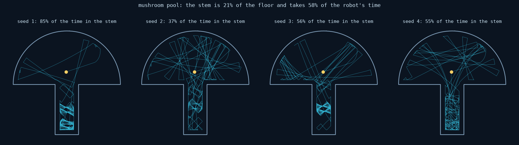
The mushroom pool. Same controller, same code, different seeds.
The stem is 21% of the floor and takes 58% of the robot's time — 85% on one
seed and 37% on another. Nothing about the algorithm causes that spread; the
room does. mushroom and stadium are pool presets chosen for their billiard
dynamics: one is a provable trap, the other provably ergodic.
The transfer operator finds the trap without being told the shape of the pool,
and the ergodic metric catches something coverage
structurally cannot — lawnmower_oracle achieves the best distribution of any
controller at twelve minutes, then finishes, parks, and spends the rest of the
cycle making it worse.
Predictions this exercise proved wrong are written up in behaviour, because they were made in public first.
Scale it
zimablue run     kidney --record runs/kidney.zbr      # a bundled scenario
zimablue run     scenarios/autumn_kidney.yaml         # or your own file
zimablue batch   kidney --episodes 100 --out results.json
zimablue compare --pool kidney --minutes 20 --jobs 4  # the planner leaderboard
A scenario is YAML: pool, robot, dirt, controller, seed, duration, termination. Batches vary the seed and aggregate, keeping enough metadata to reproduce any individual failure exactly.
Extend it
Commercial pool cleaners are evaluated by driving them around a real pool with real dirt: slow, expensive, impossible to repeat. Meanwhile Gazebo, MuJoCo and Isaac Sim each make their engine the API, so anything pool-specific you build cannot outlive the engine.
Here the domain model is the API. Pools, dirt, cleaners, scenarios, recordings and metrics are ZimaBlue concepts. Whatever integrates the equations sits behind an interface and can be swapped — today it is a deterministic CPU-only 2D backend running at 25–30× real time on one core.
                         ZimaBlue domain API
                                 │
              ┌──────────────────┼──────────────────┐
        World model         Robot model         Controller
     pool · water · dirt   body · sensors      (replaceable)
              └──────────────────┼──────────────────┘
                                 │
                        SimulationBackend
                                 │
                  ┌──────────────┴──────────────┐
             Fast2DBackend                IsaacSimBackend
              (CPU, today)                  (planned)
                                 │
                    Recording · Replay · Metrics
A backend owns dynamics and sensing, nothing else. Dirt accounting, metrics and
recording are computed by shared code from the state it returns, so a new
backend inherits them and cannot redefine how they are measured. A .zbr
written by the 3D backend will have to replay in the 2D viewer; that is the
acceptance test.
Pools, robots, dirt, controllers and backends are all registries, so adding one
means writing a function. Issues and pull requests welcome — see
CONTRIBUTING.md, which is mostly about not breaking
determinism and preferring a small real model to a large fake one.
Read more
| Getting started | Install, first run, common tasks |
| From a photo | Tracing a pool out of a picture, and what a picture cannot tell you |
| Machine learning | SAM for the water mask, Gymnasium for the controller |
| On a robot | Running a controller on real hardware, and testing it against real logs |
| Coverage path planning | The planners, the map they needed, and how to compare them |
| Benchmark | The frozen suite: one command, the same numbers |
| Fleets | Several robots in one pool: partitioning, cooperation, and what a second robot is worth |
| Behaviour | Periodic orbits, mixing rates, the ergodic metric, and pools chosen for their dynamics |
| Architecture | Layering, backends, determinism contract |
| Research | Prior art, and which decision each finding drove |
| References | Verified bibliography, with what the code implements |
| Scenarios | YAML experiments and batch sweeps |
| Recording | The .zbr format, channel by channel |
| Replay | Controls, exporters, rendering notes |
| Roadmap | Done, next, and deliberately not planned |
| Releasing | Publishing to TestPyPI and PyPI |
Examples
Every one takes --minutes if you want a shorter run.
basic.py |
The smallest useful program: pool in, metrics out |
custom_pool.py |
Build a pool from geometry, depth models and features, then read the spatial metrics |
pool_from_photo.py |
Trace a pool out of a photograph, check the trace, then clean it — --sam to segment with a model |
rl_env.py |
The Gymnasium env, and the baseline a trained policy has to beat |
live_training.py |
Watch cross-entropy policy search try candidates and improve its reward live |
tune_controller.py |
Search the shipped controller's parameters, which is the cheap thing to try first |
train_policy.py |
Train a controller with PPO, score it against the shipped ones, and replay it |
custom_robot.py |
Compose a cleaner from components and break a sensor on purpose |
custom_controller.py |
Write an autonomy stack and benchmark it against the shipped ones |
estimation_replay.py |
The EKF controller, with the pose estimate drawn against ground truth |
batch_experiment.py |
Run a scenario across seeds, then reproduce its worst episode exactly |
replay.py |
Replay a recording flat, in 3D, from the bumper, or interactively |
replay_real_trajectory.py |
Score the estimator against a real robot's logged trajectory |
fleet.py |
Several cleaners in one pool, the fleet views, and what each extra robot buys |
compare_planners.py |
Every coverage planner on every pool, scored on every axis, with the matrix plot |
analyse_dynamics.py |
Periodic orbits, mixing rates, the ergodic metric and sensitivity, for one pool |
tour.ipynb |
All of the above in one notebook, with the pool turnable in the browser |
Did you know?
That sharp "chlorine" smell at a busy pool is mostly not chlorine, and the red stinging eyes are not chlorine's fault either. Chlorine reacts with what swimmers bring in with them — sweat, skin cells, sunscreen, and yes, pee — and the chloramines that come out of the reaction are what you smell and what stings. A pool that reeks is a pool that has been swum in. So shower first, and use the toilet before you get in.
ZimaBlue models sand, algae, biofilm and leaves. Swimmers are out of scope. (CDC)
License
MIT.
1 maintainer

Metadata
1 maintainer
Release files for zimablue 0.5.0
For a detailed explanation of source distributions (sdists) and built distributions (wheels), please see the package formats documentation.
Source distribution (sdist)
| File | Size | Uploaded | |
|---|---|---|---|
| zimablue-0.5.0.tar.gz | 651.2 kB | Details |
Built distribution (wheel)
| File | Interpreter | ABI | Platform | Reset |
|---|---|---|---|---|
| zimablue-0.5.0-py3-none-any.whl | Python 3 | none | any | Details |
Total release size: 1.1 MB
Release files / zimablue-0.5.0.tar.gz
| Download URL | zimablue-0.5.0.tar.gz |
|---|---|
| Size | 651.2 kB |
| Tags | Source |
|
SHA-256 checksum How to use checksums |
3ce4e4439d2e7c84cb3d452335a003dfb5644e3aa63263689981422ee18d080b
|
|
BLAKE2b-256 checksum How to use checksums |
2fa3fadc6103083d55bc659537a197e79baa3bcde4a9808df0b203927173b0ed
|
| Upload date | |
|
Uploaded using Trusted Publishing? What is trusted publishing? |
Yes |
| Uploaded via |
twine/7.0.0 CPython/3.13.14
|
Provenance
Provenance describes where a file came from. On PyPI, provenance is shared via attestations, which provide a verifiable record of the build or publishing details. View details, limitations and caveats.


PyPI Publish Attestation
PyPI verified that this artifact, at this checksum, originated from the publisher listed below.
Signed by GitHub Actions, verified by PyPI on Aug 27, 2026.
Transparency logRelease files / zimablue-0.5.0-py3-none-any.whl
| Download URL | zimablue-0.5.0-py3-none-any.whl |
|---|---|
| Size | 439.6 kB |
| Tags | Python 3 |
|
SHA-256 checksum How to use checksums |
36ddc9a804adc2e8ddb090aa752c558ea4bf28283ff696f68f3181531f327048
|
|
BLAKE2b-256 checksum How to use checksums |
e211b51ea76e8095c66bf265c8a2d66a14c1afe27cfe2cf727beffc8dbcf0b0f
|
| Upload date | |
|
Uploaded using Trusted Publishing? What is trusted publishing? |
Yes |
| Uploaded via |
twine/7.0.0 CPython/3.13.14
|
Provenance
Provenance describes where a file came from. On PyPI, provenance is shared via attestations, which provide a verifiable record of the build or publishing details. View details, limitations and caveats.
PyPI Publish Attestation
PyPI verified that this artifact, at this checksum, originated from the publisher listed below.
Signed by GitHub Actions, verified by PyPI on Aug 27, 2026.
Transparency log













