






FluxFEM
A weak-form-centric differentiable finite element framework in JAX, where variational forms are treated as first-class, differentiable programs.
Examples and Features
| Example 1: Diffusion | Example 2: Neo-Hookean Hyper Elasticity |
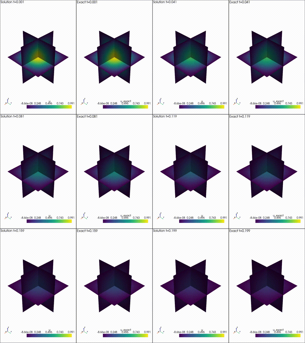
|
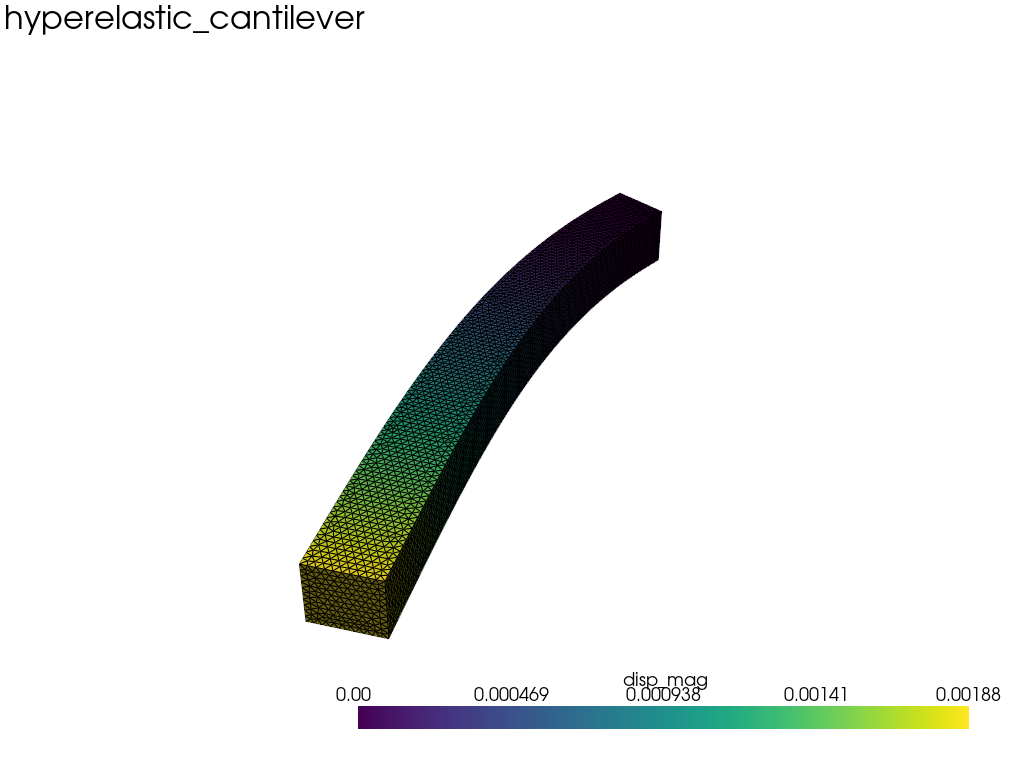
|
Features
- Built on JAX, enabling automatic differentiation with grad, jit, vmap, and related transformations.
- Weak-form–centric API that keeps formulations close to code; weak forms are represented as expression trees and compiled into element kernels, enabling automatic differentiation of residuals, tangents, and objectives.
- Two assembly approaches: tensor-based (scikit-fem–style) assembly and weak-form-based assembly.
- Handles both linear and nonlinear analyses with AD in JAX.
- Optional PETSc/PETSc-shell solvers via
petsc4pyfor scalable linear solves (addfluxfem[petsc]). - Contact interface support for penalty/constraint contact formulations, including role-explicit contact specs (
ContactSpaces,ContactGroupSpaces,OneSidedContactSpaces) and KKT assembly utilities (assemble_contact_coupling_matrices,assemble_contact_kkt,solve_contact_kkt). - Craig-Bampton ROM workflows for assembled FE systems, retained contact/interface DOFs, and fixture-style RBE3 MPC/preload or prescribed-reference models.
Usage
This library provides two assembly approaches.
- A tensor-based assembly, where trial and test functions are represented explicitly as element-level tensors and assembled accordingly (in the style of scikit-fem).
- A weak-form-based assembly, where the variational form is written symbolically and compiled before assembly.
The two approaches are functionally equivalent and share the same element-level execution model,
but they differ in how you author the weak form. The example below mirrors the paper's diffusion
case and makes the distinction explicit with jnp.
Assembly Flow
All expressions are first compiled into an element-level evaluation plan, which operates on quadrature-point–major tensors. This plan is then executed independently for each element during assembly.
As a result, both assembly approaches:
- use the same quadrature-major (q, a, i) data layout,
- perform element-local tensor contractions,
- and are fully compatible with JAX transformations such as
jit,vmap, and automatic differentiation.
kernel-based assembly (explicit JIT units)
If you want to control JIT boundaries explicitly, build a JIT-compiled element kernel
and pass it to space.assemble. The kernel must return the integrated element
contribution (not the quadrature integrand). For untagged raw kernels, pass kind=.
import fluxfem as ff
import jax
import jax.numpy as jnp

space = ff.make_hex_space(mesh, dim=1, intorder=2)

# bilinear: kernel(ctx) -> (n_ldofs, n_ldofs)
ker_K = ff.make_element_bilinear_kernel(ff.diffusion_form, 1.0, jit=True)
K = space.assemble(ff.diffusion_form, 1.0, kernel=ker_K)

# linear: kernel(ctx) -> (n_ldofs,)
def linear_kernel(ctx):
    integrand = ff.scalar_body_force_form(ctx, 2.0)
    wJ = ctx.w * ctx.test.detJ
    return (integrand * wJ[:, None]).sum(axis=0)

ker_F = jax.jit(linear_kernel)
F = space.assemble(ff.scalar_body_force_form, 2.0, kernel=ker_F)
tensor-based vs weak-form-based (diffusion example)
tensor-based assembly
The tensor-based assembly provides an explicit, low-level formulation with element kernels written using jax.numpy.(jnp).
import fluxfem as ff
import jax.numpy as jnp

@ff.kernel(kind="bilinear", domain="volume")
def diffusion_kernel(ctx: ff.FormContext, kappa):
    # ctx.test.gradN / ctx.trial.gradN: (n_qp, n_nodes, dim)
    # output tensor: (n_qp, n_nodes, n_nodes)
    return kappa * jnp.einsum("qia,qja->qij", ctx.test.gradN, ctx.trial.gradN)

space = ff.make_hex_space(mesh, dim=3, intorder=2)
params = ff.Params(kappa=1.0)
K_ts = space.assemble(diffusion_kernel, params=params.kappa)
weak-form-based assembly
In the weak-form-based assembly, the variational formulation itself is the primary object. The expression below defines a symbolic weak form. FluxFEM compiles it internally during assembly, and you can still request an explicit compiled object when you want reuse/control.
import fluxfem as ff
import fluxfem.helpers_wf as h_wf

space = ff.make_hex_space(mesh, dim=3, intorder=2)
params = ff.Params(kappa=1.0)
U = ff.NamedSpace("U", space)
V = ff.NamedSpace("V", space)

# u, v are symbolic trial/test fields (weak-form DSL objects).
# u.grad / v.grad are symbolic nodes (expression tree), not numeric arrays.
form_wf = ff.BilinearForm.volume(
    lambda u, v, p: p.kappa * (v.grad @ u.grad) * h_wf.dOmega()
)

# Shortest path for standard Galerkin assembly (U == V == space).
K_wf = space.assemble(form_wf, params=params)

# Equivalent explicit-role form when you want U/V to appear in the code.
K_wf_roles = ff.BilinearSpaces(test=V, trial=U).assemble(form_wf, params=params)
If you want to compile once and reuse explicitly:
compiled = ff.BilinearForm.volume(
    lambda u, v, p: p.kappa * (v.grad @ u.grad) * h_wf.dOmega()
).get_compiled()

K_wf = space.assemble(compiled, params=params)
Linear Elasticity assembly (weak-form based assembly)
import fluxfem as ff
import fluxfem.helpers_wf as h_wf

space = ff.make_hex_space(mesh, dim=3, intorder=2)
D = ff.isotropic_3d_D(1.0, 0.3)

form_wf = ff.BilinearForm.volume(
    lambda u, v, D: h_wf.ddot(v.sym_grad, D @ u.sym_grad) * h_wf.dOmega()
)

K = space.assemble(form_wf, params=D)
Neo-Hookean residual assembly (weak-form DSL)
Below is a Neo-Hookean hyperelasticity example written in weak form. The residual is expressed symbolically and compiled into element-level kernels executed per element. No manual derivation of tangent operators is required; consistent tangents (Jacobians) for Newton-type solvers are obtained automatically via JAX AD.
def neo_hookean_residual_wf(v, u, params):
    mu = params["mu"]
    lam = params["lam"]
    F = h_wf.I(3) + h_wf.grad(u)  # deformation gradient
    C = h_wf.matmul(h_wf.transpose(F), F)
    C_inv = h_wf.inv(C)
    J = h_wf.det(F)

    S = mu * (h_wf.I(3) - C_inv) + lam * h_wf.log(J) * C_inv
    dE = 0.5 * (h_wf.matmul(h_wf.grad(v), F) + h_wf.transpose(h_wf.matmul(h_wf.grad(v), F)))
    return h_wf.ddot(S, dE) * h_wf.dOmega()

res_form = ff.ResidualForm.volume(neo_hookean_residual_wf)
R = space.assemble_residual(res_form, u, ff.Params(mu=1.0, lam=1.0))
J = space.assemble_jacobian(res_form, u, ff.Params(mu=1.0, lam=1.0))
autodiff + jit compile
You can differentiate through the solve and JIT compile the hot path. The inverse diffusion tutorial shows this pattern:
def loss_theta(theta):
    kappa = jnp.exp(theta)
    u = solve_u_jit(kappa, traction_true)
    diff = u[obs_idx_j] - u_obs[obs_idx_j]
    return 0.5 * jnp.mean(diff * diff)

solve_u_jit = jax.jit(solve_u)
loss_theta_jit = jax.jit(loss_theta)
grad_fn = jax.jit(jax.grad(loss_theta))
FESpace vs FESpacePytree
Use FESpace for standard workflows with a fixed mesh. When you need to carry
the space through JAX transformations (e.g., shape optimization where mesh
coordinates are part of the computation), use FESpacePytree via
make_*_space_pytree(...). This keeps the mesh/basis in the pytree so
jax.jit/jax.grad can see geometry changes.
In other words:
- fixed-geometry solve/assembly:
FESpace - geometry-sensitive differentiation:
FESpacePytree
The mesh-move example in tutorials/diffusion/diffusion_3d_mesh_proxy.py
computes jax.grad(...) with respect to node coordinates on top of
make_hex_space_pytree(...).
Current boundary:
- geometry-dependent objectives and residual-style quantities can be differentiated in JAX when the geometry is carried through a pytree space
- there is not yet a dedicated public "shape derivative" API layer; shape sensitivity is currently expressed as ordinary JAX differentiation through assembly/solve code
backend="numpy"is not part of this differentiable path
For same-space Galerkin assembly, space.assemble(...) and space.assemble_*
remain the shortest paths.
When you want the roles to be explicit, prefer
LinearSpaces(...).assemble(...), BilinearSpaces(...).assemble(...),
ResidualSpaces(...).assemble(...), and JacobianSpaces(...).assemble(...).
For contact interfaces, prefer contact.assemble_* methods over top-level
ff.assemble_contact_* helpers. The top-level assemble_* helpers remain
available as compatibility entrypoints.
Structural beam/truss helpers
FluxFEM also includes dedicated structural-element helpers for quick beam,
bar/truss, and lumped spring-mass-dashpot models. These are separate from the
continuum FESpace mesh assembly path:
- frame2d: x-z planar Euler-Bernoulli frame elements, 3 DOF per node (
ux, uz, ry) - beam: 3D Euler-Bernoulli frame elements, 6 DOF per node
- truss2d/bar: x-z planar axial elements, 2 translational DOF per node
- truss/bar: 3D axial elements, 3 translational DOF per node
- lumped: DOF-level springs, dashpots, nodal loads, and Rayleigh damping
Matrix assembly uses an explicit return format:
format="csr": SciPy CSR matrix, the defaultformat="fluxsparse":FluxSparseMatrix, useful with JAX-oriented sparse solvesformat="dense": NumPy dense matrix for small checks
Load vectors are dense and can choose array_backend="numpy" or
array_backend="jax" when needed.
coords, conn = ff.structured_beam_chain(n_elems=8, length=2.0)
section = ff.BeamSection(E=210e9, G=80e9, A=2e-3, Iy=8e-6, Iz=5e-6, J=1e-5)

K = ff.assemble_beam_stiffness(coords, conn, section, format="csr")
F = ff.assemble_beam_point_load(coords.shape[0], coords.shape[0] - 1, force=(0.0, 0.0, -1000.0))
fixed = ff.beam_node_dofs([0])

u, info = ff.LinearSolver(method="spsolve").solve(
    K,
    F,
    dirichlet=ff.DirichletBC(fixed, 0.0),
    dirichlet_mode="condense",
)
For a JAX sparse-style path, request format="fluxsparse" and a JAX RHS:
K = ff.assemble_truss_stiffness(coords, conn, truss_section, format="fluxsparse")
F = ff.assemble_truss_point_load(n_nodes, tip_node, force=(1200.0, 0.0, 0.0), array_backend="jax")
u, info = ff.LinearSolver(method="spsolve_jax").solve(K, F, dirichlet=bc)
For coupled structural models, NumpyCoupledSystemBuilder and
JAXCoupledSystemBuilder provide add_dof_tie_constraint(...) to tie selected
field-local DOFs, for example a 6-DOF beam root to a 6-DOF remote point.
They also provide add_distributed_coupling(...) for weighted face/patch-to-
remote distributed coupling and add_bolt_preload(...) for directional remote
preload springs. The distributed coupling is RBE3-style weighted least-squares
remote reconstruction, validates 6-DOF patch rank by default, and is not a full
Nastran RBE3 card-compatible implementation. Its generated RBE3 rows are tested
for force and moment balance by virtual work. It supports dependent reference
component selection through dependent_components, so translational-only
couplings are assembled without remote-rotation columns and do not require a
full 6-DOF patch rank. RBE2 helpers also support slave translation component
selection through slave_components.
Plate/shell helpers include Q4 Mindlin/Reissner-Mindlin plate elements and
linear Q4 Reissner-Mindlin shell elements. Shells use 6 DOF/node and can be
assembled on 2D flat coordinates or 3D planar element coordinates. Plate and
shell sections expose shear_mode="reduced" | "full" | "mitc4" and rho for
consistent mass assembly; the default keeps the existing selective reduced
shear integration, while mitc4 uses an edge-tying assumed-shear variant for
locking/hourglass studies. Solid-shell examples cover coincident-node
translational ties and solid-patch-to-shell-edge RBE3 remote coupling.
Nonmatching planar shell-solid translational ties are available through solid
surface facet interpolation; see
notes/plate_shell_status.md for current limits.
Nonlinear material support currently centers on compressible Neo-Hookean
hyperelasticity through JAX AD residual/Jacobian assembly. A small-strain J2
plasticity material-point return mapping and FE-facing frozen-state residual /
quadrature update helpers are available. The J2 load-step helper commits
quadrature histories after converged steps, supports displacement and external
load scaling, and exposes per-step Newton iteration diagnostics for convergence
checks. Quadrature strain/stress diagnostics are exposed for verification, with
tests covering material-point references, unload/reload elastic increments,
force-controlled elastic loading, mixed-BC plastic loading, and small multi-hex
step-refinement consistency. tutorials/nonlinear/j2_uniaxial_tension.py
writes VTU cell data, a CSV load history, and a Newton iteration CSV for full
displacement, mixed-BC, or small force-controlled J2 bar examples. Production
restart/output and general lifecycle management for plasticity, continuum
viscoelasticity, and damage are not mature yet; see
notes/material_models_status.md for the current scope and recommended next
steps.
Backend support summary for the structural helpers:
| Feature | SciPy/NumPy path | JAX path | Notes |
|---|---|---|---|
| Beam / frame / truss assembly | format="csr" or "dense" |
format="fluxsparse" and JAX load vectors |
Older `backend="scipy" |
| Mindlin plate / Reissner-Mindlin shell assembly | format="csr" or "dense" |
format="fluxsparse" and JAX load vectors |
Stiffness and mass matrices share the same backend path; mass requires section.rho. |
| DOF ties, RBE2, RBE3, distributed coupling, bolt preload | NumpyCoupledSystemBuilder |
JAXCoupledSystemBuilder |
Tests compare representative NumPy and JAX builder results. |
| Shell-solid coincident tie | NumpyCoupledSystemBuilder tutorials |
Constraint rows are compatible with JAXCoupledSystemBuilder |
Translational shell DOFs only. |
| Shell-solid nonmatching tie | CSR constraint matrix for NumPy builder | Dense/JAX-array constraint matrix for JAX builder | Node-to-surface interpolation on planar tri/quad facets; not mortar. |
| Contact and mortar workflows | Mixed: many setup/reference paths use NumPy/SciPy | JAX is the primary AD/Jacobian path | Contact backend support is more specialized than the structural helpers. |
See:
tutorials/elasticity/beam_cantilever.pytutorials/elasticity/frame2d_cantilever.pytutorials/elasticity/beam_uniform_load.pytutorials/elasticity/solid_beam_rbe3_coupling.pytutorials/elasticity/truss2d_bar_cantilever.pytutorials/elasticity/truss_bar_cantilever.pytutorials/elasticity/solid_truss_rbe3_coupling.pytutorials/dynamics/beam_tip_spring_dashpot.py
Mixed systems
Mixed systems use two kinds of names:
- field name: the global block name in the mixed vector, such as
"u"or"p" - FE space: the discrete space where that field lives
Start from the mathematical picture:
- unknown
ulives in FE spaceV - unknown
plives in FE spaceQ
V = ff.make_hex_space(mesh, dim=3, intorder=2)
Q = ff.make_hex_space(mesh, dim=1, intorder=2)

# "u in V"  (the name "u" is the mixed field name)
u_field = ff.NamedSpace("u", V)

# "p in Q"
p_field = ff.NamedSpace("p", Q)

mixed = ff.MixedSpace(u_field, p_field)
Read that as:
"u"and"p"are the field names in the global mixed vectorVandQare the actual FE spaces for those fields
So ff.NamedSpace("u", V) means:
- this mixed field is called
"u" - it lives in FE space
V
In the common mixed API, field names are also the default symbolic names used inside weak forms. That keeps the notation close to the mathematical picture.
If you want to make the per-field roles explicit, MixedSpace(...) can also
reuse the existing single-field role specs:
U = ff.NamedSpace("u", V)
Vt = ff.NamedSpace("v_u", V)
P = ff.NamedSpace("p", Q)
Qt = ff.NamedSpace("v_p", Q)

mixed = ff.MixedSpace(
    u=ff.ResidualSpaces(test=Vt, unknown=U),
    p=ff.BilinearSpaces(test=Qt, trial=P),
)
That reads as:
- the
ufield usesVfor both test and unknown, with explicit symbolic namesv_uandu - the
pfield usesQfor both test and trial, with explicit symbolic namesv_pandp
Next, define one residual function per equation. Inside those functions, use the
field names when you want to refer to another unknown symbolically.
Here unknown_ref("p") means "the symbolic mixed unknown stored under field name p".
The test function is usually just the first local argument (v, q), so a separate
test-side lookup is often unnecessary.
def res_u(v, u, p):
    p_ref = ff.unknown_ref("p")
    return (...) * h_wf.dOmega()

def res_p(q, p_field, p):
    u_ref = ff.unknown_ref("u")
    return (...) * h_wf.dOmega()
For the common case where residual names and field names match, keep it short:
residuals = ff.make_mixed_residuals(
    u=res_u,
    p=res_p,
)
If you need to route an equation to a different field name explicitly, use
bind_mixed_residual(...).
Once the field layout and residual bindings are defined, assembly follows the same object-centered flow as the single-space API:
res_form = ff.ResidualForm.mixed(residuals)
R = mixed.assemble_residual(res_form, u0, ff.Params(alpha=1.0))
J = mixed.assemble_jacobian(res_form, u0, ff.Params(alpha=1.0))
If you prefer a higher-level problem object, MixedProblem(...) is still available.
Contact weak forms
Contact follows the same broad assembly pattern as the volume and surface APIs:
- define a contact spec
- prepare a reusable interface object
- optionally update a contact state at the current iterate
- assemble interface operators or contact contributions
The main difference from standard volume assembly is that contact has a state-dependent geometric part. In FluxFEM terms:
ContactPairSpec/ContactGroupSpec/OneSidedContactSpecare declarative specsprepare(...)performs the heavy reusable setupinitialize_state()/update_state(...)expose the state-explicit nonlinear path
FluxFEM contact assembly is expressed in residual/jacobian form. When comparing
against references written directly as K u = f bilinear/linear forms, a global
sign flip may be required to match conventions; this is expected if the physics
is otherwise identical.
In the current implementation, prepare(...) is the preferred public alias for
the older to_contact_surface_space(...) setup step.
Pair Contact Quickstart
Start by defining a contact side on each body, then combine them into a contact spec and prepare a reusable interface:
master_side = ff.ContactSideSpec.from_facets(master_mesh, master_facets, master_space)
slave_side = ff.ContactSideSpec.from_facets(slave_mesh, slave_facets, slave_space)

contact = ff.ContactPairSpec(
    master=master_side,
    slave=slave_side,
).prepare(
    quad_order=1,
    backend="jax",
)
Internally, this setup step prepares reusable interface data such as pairing, supermesh geometry, facet-to-element maps, and quadrature caches.
Once you have a prepared contact interface, bilinear weak forms follow the same object-centered pattern:
contact_form = ff.BilinearForm.contact(a_contact)
B = contact.assemble_bilinear_form(contact_form, params)
If you want an explicit compiled object for reuse:
compiled = ff.BilinearForm.contact(a_contact).get_compiled()
B = contact.assemble_bilinear_form(compiled, params)
State-Explicit Nonlinear Contact
For curved surfaces, load stepping, or nonlinear contact updates, expose the state-dependent part explicitly:
contact_state = contact.initialize_state()

contact_state = contact.update_state(
    state={"a": u_master, "b": u_slave},
    contact_state=contact_state,
    geometry="current",
    active_set="update",
)
The current ContactState object is a lightweight public skeleton for this
workflow. It records the interface kind, iteration, geometry mode, and a shape
summary of the current field state. This is the intended public boundary for
future state-dependent contact updates.
Penalty Contact
Penalty-family contact assembly uses the same prepared contact object:
ops_penalty = contact.assemble_penalty(
    weak_form=contact_residual_form,
    state={"a": u_master, "b": u_slave},
    params=params,
    backend="jax",
)
Multiplier Contact
Constraint-family contact adds a multiplier spec on top of the same interface:
lm_space = ff.MultiplierSpec.dual_mortar()

ops_constraint = contact.assemble_multiplier(
    rho=1.0,
    multiplier=lm_space,
    backend="numpy",
)
So the usual flow is:
- create
ContactSideSpecobjects from mesh facets - build a spec with
ContactPairSpec(...) - call
prepare(...)to build reusable interface setup - optionally call
initialize_state()/update_state(...)in nonlinear loops - choose penalty or multiplier assembly on that prepared contact object
Mixed weak-form naming follows this convention:
- simple single-space code:
ctx.test/ctx.trial - named mixed field lookup:
ctx.bindings["u"] - explicit space-key lookup:
ctx.spaces["V"] - explicit residual-to-field routing:
bind_mixed_residual(...)
Use the explicit forms only where they help readability or avoid ambiguity. Examples:
tutorials/diffusion/coupled_reaction_diffusion_new_api.pytutorials/diffusion/ch3d_fluxfem_wf_new_api.pytutorials/diffusion/carburizing_diffusion_bar.py(transient carbon diffusion / heat-treatment style example)
Backend notes
backend="jax" is the primary path for differentiation and Jacobian assembly.
backend="numpy" is available mainly for forward assembly/evaluation and comparison/debug workflows.
Today, the practical split is:
jax: bilinear/linear/residual assembly, autodiff-based Jacobians, geometry-sensitive differentiationnumpy: bilinear/linear/residual/functional forward assembly in many paths, plus several contact/coupled utilitiesnumpyJacobian assembly is not generally implemented; for exampleassemble_jacobian(..., backend="numpy")is not available
For contact/supermesh code, backend="numpy" is also used in places where the Jacobian is approximated by finite differences rather than differentiated symbolically.
Block assembly
For constraints like contact problems (e.g., adding Lagrange multipliers), build a block matrix explicitly:
from fluxfem import solver as ff_solver

# Example blocks from contact coupling
K_uu = ...
K_cc = ...
K_uc = ...

blocks = ff_solver.make_block_matrix(
    diag=ff_solver.block_diag(order=("u", "c"), u=K_uu, c=K_cc),
    rel={("u", "c"): K_uc},
    symmetric=True,
    transpose_rule="T",
)

# Lazy container; assemble when you need the global matrix.
K = blocks.assemble()
FluxFEM also provides high-level contact utilities:
# Pair contact
side_master = ff.ContactSideSpec.from_surfaces(surf_master, elem_conn=conn_master, value_dim=3)
side_slave = ff.ContactSideSpec.from_surfaces(surf_slave, elem_conn=conn_slave, value_dim=3)
contact = ff.ContactPairSpec(master=side_master, slave=side_slave).prepare(
    quad_order=4,
    backend="jax",
)

# One-to-many contact
contact_group = ff.ContactGroupSpec(
    master=side_master,
    slaves=[side_slave],
).prepare(
    quad_order=4,
    backend="jax",
)

# One-sided contact
floor_contact = ff.OneSidedContactSpec(side=side_slave).prepare(
    quad_order=4,
)

# Optional nonlinear/state-explicit update
contact_state = contact.initialize_state()
contact_state = contact.update_state(
    state={"a": u_master, "b": u_slave},
    contact_state=contact_state,
    geometry="current",
    active_set="update",
)

# 1) Assemble constraint operators (B, Kuu, ...)
lm_space = ff.MultiplierSpec.coarse_dual_mortar(max_rank=64)

ops: ff.ContactOperators = contact_group.assemble_multiplier(
    rho=1.0,
    multiplier=lm_space,
    backend="numpy",
    # Optional: also evaluate and store residual/jacobian metadata on the same ContactOperators.
    weak_form=contact_residual_form,
    state={"a": u_master, "b": u_slave},
    params=params,
)

# 2) Penalty-family path: user weak form -> residual/jacobian operators
ops_nitsche: ff.ContactOperators = contact.assemble_penalty(
    weak_form=contact_residual_form,
    state={"a": u_master, "b": u_slave},
    params=params,
    backend="jax",
)

# 3) Unified coupled API (Penalty Family)
builder = ff.CoupledSystemBuilder.from_structural(K_u, F_u)
builder.register_blocks([
    ("master", space_master, {"value_dim": 1}),
    ("slave", space_slave, {"value_dim": 1}),
])
builder.add_contact(
    ops_nitsche,
    master="master",
    slave="slave",
    value_dim=1,
)
system = builder.build()
u = system.solve(dirichlet_dofs=dir_dofs, dirichlet_vals=0.0, format="csr")

# 4) Unified coupled API (Constraint Family): KKT assembly is internal to builder
builder_mortar = ff.CoupledSystemBuilder.from_structural(K_u, F_u)
builder_mortar.register_blocks([
    ("master", space_master, {"value_dim": 1}),
    ("slave", space_slave, {"value_dim": 1}),
])
builder_mortar.add_contact(
    ops,
    master="master",
    slave="slave",
    value_dim=1,
)
system_mortar = builder_mortar.build()

# Or let the builder assemble the mortar operators from a prepared contact.
builder_mortar.add_contact(
    contact_group,
    master="master",
    slave="slave",
    family="constraint",
    mortar="coarse_dual",
    rho=1.0,
    value_dim=1,
)

# Advanced: law/formulation can be set explicitly when needed.
# - law="one_sided_normal_frictionless"
# - formulation="multiplier" | "penalty_consistent"
Contact API boundaries (fixed terms):
spec: declarative contact definition (ContactPairSpec,ContactGroupSpec,OneSidedContactSpec).contact: prepared interface geometry/pairing/supermesh/quadrature.contact_state: current-iterate contact state for nonlinear workflows.multiplier: LM discretization (family,side,value_dim).formulation: enforcement variant used for routing.ops: assembled bundle passed toCoupledSystemBuilder.
Notes:
- Multiple contacts can be added with different settings per
builder.add_contact(...)call. prepare(...)is the preferred public name for the reusable setup step;to_contact_surface_space(...)remains available as a compatibility entrypoint.ContactStatecurrently provides the public skeleton for state-explicit contact workflows; future nonlinear contact updates should build on this boundary.MultiplierSpecis the preferred public name for multiplier discretization;ContactMultiplierSpaceremains available as a compatibility name.MultiplierSpec()defaults tofamily="dual_nodal"for mortar, giving a master-side dual nodal map withB_a = IandB_b = pinv(M_aa) M_ab; passfamily="nodal"to recover the original nodal multiplier basis.- Common mortar choices have factory constructors:
MultiplierSpec.dual_mortar(),MultiplierSpec.coarse_dual_mortar()for algebraic SVD/QR row reduction,MultiplierSpec.nodal_mortar(),MultiplierSpec.p0_mortar(contact),MultiplierSpec.coarse_p0_mortar(contact, patch_ids=...)for integrated P0 patch grouping, andMultiplierSpec.coarse_p1_mortar(basis=C)for integrated coarse P1 rowsC @ M; build simpleCmatrices withcoarse_p1_basis_from_node_groups(...)orcoarse_p1_basis_from_surface_grid(...). solve_augmented_lagrangian_outer_loop(...)provides a low-level AL loop around user-supplied inner solves and eitherconstraint_fn(solution)orContactOperators.B @ solution - offset.ContactMultiplierSpace/MultiplierSpecp0-like families ("p0","p0_active","p0_supermesh") currently supportside="master"only.- See docs:
Usage -> Contact API Boundaries.
Documentation
Full documentation, tutorials, and API reference are hosted at this site.
Tutorials
tutorials/elasticity/linearelastic_tensile_bar.py(linear elasticity, weak-form assembly)tutorials/elasticity/frame2d_cantilever.py,tutorials/elasticity/beam_cantilever.py, andtutorials/elasticity/beam_uniform_load.py(2D/3D Euler-Bernoulli frame helpers)tutorials/elasticity/mindlin_plate_cantilever.py(Q4 Reissner-Mindlin/Mindlin plate helper,--shear-mode reduced|full|mitc4)tutorials/elasticity/mindlin_plate_shear_locking_benchmark.py(thin-plate shear locking comparison forfull,reduced, andmitc4)tutorials/elasticity/flat_shell_cantilever.py(Q4 Reissner-Mindlin shell helper, 2D/tilted 3D coordinates,--shear-mode reduced|full|mitc4, and optional VTU output)tutorials/elasticity/flat_shell_shear_locking_benchmark.py(thin-shell shear locking comparison and tilted 3D frame check)tutorials/elasticity/solid_shell_translational_tie.py(solid surface tied to a shell skin by translational DOFs,--shear-mode reduced|full|mitc4)tutorials/elasticity/solid_shell_nonmatching_tie.py(nonmatching shell nodes tied to interpolated solid surface translations)tutorials/elasticity/solid_shell_rbe3_patch_coupling.py(solid face patch coupled to a shell root edge through a 6-DOF RBE3 remote point,--shear-mode reduced|full|mitc4)tutorials/elasticity/shell_solid_cantilever_benchmark.py(shell and solid cantilever comparison against an Euler-Bernoulli estimate,--shear-mode reduced|full|mitc4)tutorials/elasticity/solid_beam_rbe3_coupling.py(3D continuum face coupled to a 3D beam root through RBE3)tutorials/elasticity/truss2d_bar_cantilever.py,tutorials/elasticity/truss_bar_cantilever.py, andtutorials/elasticity/truss_uniform_load.py(2D/3D truss/bar helpers)tutorials/elasticity/solid_truss_rbe3_coupling.py(3D continuum face coupled to a 3D truss/bar root through RBE3)tutorials/dynamics/spring_mass_dashpot.pyandtutorials/dynamics/beam_tip_spring_dashpot.py(lumped and beam dynamics)tutorials/nonlinear/neo_hookean_cantilever.py(nonlinear hyperelasticity)tutorials/thermoelastic/thermoelastic_bar_1d.py/tutorials/thermoelastic/thermoelastic_bar_1d_mixed.py(thermoelastic coupling)tutorials/contact/contact_supported_box_by_truss_springs.py(3D contact pad backed by truss-equivalent support springs)tutorials/contact/contact_supported_box_by_pillars.py(large box supported by multiple small boxes via penalty contact + Dirichlet supports)tutorials/contact/two_body_contact_displacement_vtu.py(two-body contact solve exported as a combined VTU)tutorials/contact/contact_mortar_builder_methods.py(dual/coarse mortar multiplier selection through explicit operators and builder-managed raw contacts)tutorials/contact/mortar_fixture_workpiece_comparison.py(matching/nonmatching fixture-workpiece mortar solves, centered on coarse P1 mortar versus the dual reference)tutorials/petsc/petsc_shell_poisson_demo.py(PETSc shell solver integration; see alsotutorials/petsc/petsc_shell_poisson_pmat_demo.py)
Craig-Bampton ROM tutorials:
tutorials/craig_bampton/craig_bampton_reduced_coupled_builder.pyis the preferred compact API path: name-based structural registration,reduce_field(..., method="craig_bampton"), explicit RBE3 remote fixture fields, preload, and prescribed-reference variants.tutorials/craig_bampton/craig_bampton_multifield_builder.pyextends the same builder pattern to multiple reduced subsystems connected by named retained interface groups, including surface-derived groups, inspectable reduced contact-pair DOFs, and contact-pair parameter metadata for contact-ready interfaces.tutorials/craig_bampton/craig_bampton_two_bar_subsystems.pybuilds two larger sparse FE subsystems, reduces each one with its own CB basis, ties the retained interface, and compares against the full coupled KKT solve.tutorials/craig_bampton/reduced_equation_builder_nonlinear.pycomposes nonlinear residual equations over multiple CB-reduced fields and obtains the global reduced Jacobian through autodiff.tutorials/craig_bampton/craig_bampton_rbe3_preload_component.pyis the experiment-2 style validation tutorial. It compares full explicit-reference RBE3 KKT solves against the CB-projected ROM for preload and Dirichlet fixture boundaries, with optional rotational RBE3 reference DOFs.tutorials/craig_bampton/craig_bampton_sparse_fe_basis.pydemonstrates CB basis construction from current sparse FE matrices, sparse-preserving projection, and matrix-free reduced operator actions withproject_operator(...).tutorials/craig_bampton/craig_bampton_vibration_rom.pyprojects both stiffness and mass matrices and compares full-order and CB-ROM free-vibration frequencies.tutorials/craig_bampton/craig_bampton_plate_shell_modes.pycompares full-order and CB-ROM free-vibration frequencies for Mindlin plate and Reissner-Mindlin shell mass/stiffness matrices.tutorials/craig_bampton/craig_bampton_contact_rom.py,tutorials/craig_bampton/craig_bampton_active_contact_newmark.py, and the node/surface-quadrature contact variants demonstrate retained contact/interface DOFs with explicit active-contact updates outside the differentiated residual.tutorials/craig_bampton/craig_bampton_rbe3_preload_mpc.pyandtutorials/craig_bampton/craig_bampton_fluxfem_rbe3_preload_experiment2.pyare lower-level compatibility/reference examples usingRBE3Patch,ReferencePointFixture, and manual projection APIs.
Setup
You can install FluxFEM either via pip or Poetry.
Supported Python Versions
FluxFEM supports Python 3.11–3.13:
Choose one of the following methods:
Using pip
pip install fluxfem
pip install "fluxfem[cuda12]" -f https://storage.googleapis.com/jax-releases/jax_cuda_releases.html
Using poetry
poetry add fluxfem
poetry add fluxfem[cuda12]
PETSc Integration
Optional PETSc-based solvers are available via petsc4py. Enable with the extra:
pip install "fluxfem[petsc]"
or
pip install "fluxfem[petsc,cuda12]" -f https://storage.googleapis.com/jax-releases/jax_cuda_releases.html
poetry add fluxfem --extras "petsc"
or
poetry add "fluxfem[petsc,cuda12]"
or
poetry add fluxfem --extras "petsc" --extras "cuda12"
Note: you must match the petsc4py version to the PETSc version you have
installed. The current FluxFEM extra pins petsc4py==3.24.4 (see
[project.optional-dependencies]), so make sure your PETSc install is
compatible with that petsc4py release, or override it to match your PETSc
build.
For a custom PETSc build, install the regular Poetry environment first and then
build petsc4py against that PETSc installation:
export PETSC_DIR=/path/to/petsc-3.24.4
export PETSC_ARCH=arch-linux-c-opt
scripts/install_petsc4py
The script keeps PETSc optional: if PETSc cannot be imported, PETSc-specific
tests are skipped by petsc_is_available().
GPU note: this repo currently tests CUDA via the cuda12 extra only. Other CUDA
versions are not covered by CI and may require manual JAX installation.
Capability Snapshot
- Core FEM and assembly
- Hex/tet-style continuum spaces, weak-form DSL assembly, tensor/kernel assembly, mass assembly, Dirichlet handling, and SciPy/JAX-oriented sparse paths.
- Differentiable residual/Jacobian workflows are centered on JAX; NumPy/SciPy paths are intended for conventional assembly, sparse solves, and regression checks.
- Structural elements
- Spring/mass/dashpot and Rayleigh damping helpers.
- 2D frame, 3D Euler-Bernoulli beam, 2D/3D truss/bar helpers with stiffness, mass, point loads, and distributed/uniform loads.
- Q4 Mindlin plate and Q4 Reissner-Mindlin shell helpers with
reduced,full, andmitc4shear options.
- Coupling and constraints
- MPC-style DOF ties, rigid/RBE2-style constraints, RBE3-style distributed coupling, bolt preload, and distributed coupling rows.
- Coincident shell-solid translational ties, nonmatching shell-solid translational interpolation, solid-shell RBE3 patch coupling, solid-beam RBE3 coupling, and solid-truss RBE3 coupling.
- Direct solid-shell rotational continuity is not implemented; use shell/beam DOFs or RBE3-style patch transfer where appropriate.
- Dynamics and ROM
- Linear Newmark dynamics for assembled systems and reduced coordinates.
- Craig-Bampton ROM for assembled stiffness/mass matrices with SciPy and JAX backend coverage on structural element matrices.
- Full-vs-CB regressions cover beam, truss, plate, shell, solid-shell, solid-beam, solid-truss, and combined solid + shell + beam models.
- Mixed solid + shell + beam CB-ROM is checked for static, constrained modal, and constrained Newmark histories.
- Contact and interfaces
- Penalty contact, active contact update loops, node-surface and paired-surface contact helpers, contact diagnostics, and KKT/mortar-oriented utilities.
- Contact examples include supported boxes, two-body contact VTU output, mortar builder methods, and CB contact tutorials.
- Materials and multiphysics
- Linear elasticity, diffusion/heat examples, thermoelastic examples, Neo-Hookean hyperelastic residual examples, and J2 material-point / FE quadrature-state / basic load-step entry points are available.
- Production restart/output and general lifecycle management for plasticity, general viscoelasticity, and damage is not yet mature.
- Visualization and tutorials
- Several tutorials export VTU for inspection, including shell and contact examples.
- Some experimental contact/sphere scripts may remain outside the tracked tutorial set until their behavior is stable.
Roadmap Status
- Phase 1: structural element base
- Implemented: spring/mass/dashpot helpers, bar/truss helpers, 2D frame helpers, and 3D Euler-Bernoulli beam helpers.
- Partial / future: Timoshenko beam and geometrically nonlinear beam/frame workflows.
- Phase 2: practical constraints and coupling
- Implemented: MPC-style rows, rigid/RBE2-style constraints, RBE3-style distributed coupling, tie constraints, bolt preload, and distributed coupling.
- Note: RBE2/RBE3 helpers are tested FluxFEM-style constructions, not complete Nastran card-compatible implementations.
- Phase 3: plate, shell, and mixed-dimensional coupling
- Implemented: Q4 Mindlin/Reissner-Mindlin plate helpers, Q4 Reissner-Mindlin shell helpers, MITC4-style shear option, shell-solid translational ties, and solid-shell/beam/truss RBE3-style coupling examples.
- Partial / future: curved/general shell kinematics, drilling-DOF treatment beyond the current helper scope, layered shells, and direct shell-solid rotational continuity.
- Phase 4: contact
- Implemented: penalty-style contact helpers, active contact update loops, node/surface and paired-surface utilities, KKT/contact builder paths, mortar-oriented utilities, and contact VTU/tutorial examples.
- Partial / future: production-grade general frictional contact, robust large-sliding workflows, and full mortar contact lifecycle management.
- Phase 5: nonlinear materials
- Implemented: Neo-Hookean hyperelastic residual examples and small-strain J2 material-point / FE quadrature-state / load-step helpers with VTU, load-history CSV, Newton diagnostics, and tangent diagnostic tests.
- Partial / future: production restart/output for plasticity, damage, viscoelasticity, and broader material lifecycle APIs.
- Phase 6: optimization and ROM
- Implemented: differentiable residual/Jacobian workflows, objective differentiation through JAX paths, Craig-Bampton ROM for stiffness/mass systems, reduced Newmark utilities, and mixed solid + shell + beam CB-ROM checks.
- Partial / future: polished support-layout/shape-parameter optimization workflows, frequency-response examples, and broader nonlinear/contact ROM lifecycle tooling.
- Deferred application areas
- Not a current focus: full reinforced-concrete solver coverage, production-grade large-scale commercial-CAE feature parity, and fully general friction/wear contact.
- Possible stepping stone: embedded reinforcement / embedded truss-style modeling before domain-specific RC workflows.
Acknowledgements
I acknowledge the open-source software, libraries, and communities that made this work possible.
Citation
Reference to cite if you use FluxFEM in a paper:
@software{Watanabe_FluxFEM_2026,
author = {Watanabe, Kohei},
doi = {10.5281/zenodo.18734689},
month = {2},
title = {{FluxFEM}},
url = {https://github.com/kevin-tofu/fluxfem},
year = {2026}
}
1 maintainer

Metadata
1 maintainer
Release files for fluxfem 0.3.10
For a detailed explanation of source distributions (sdists) and built distributions (wheels), please see the package formats documentation.
Source distribution (sdist)
| File | Size | Uploaded | |
|---|---|---|---|
| fluxfem-0.3.10.tar.gz | 367.3 kB | Details |
Built distribution (wheel)
| File | Interpreter | ABI | Platform | Reset |
|---|---|---|---|---|
| fluxfem-0.3.10-py3-none-any.whl | Python 3 | none | any | Details |
Total release size: 759.8 kB
Release files / fluxfem-0.3.10.tar.gz
| Download URL | fluxfem-0.3.10.tar.gz |
|---|---|
| Size | 367.3 kB |
| Tags | Source |
|
SHA-256 checksum How to use checksums |
43bb7b1473aa9e3ceb23f109ebc884c63ea9a455a399c845e190f2e2dad297cd
|
|
BLAKE2b-256 checksum How to use checksums |
4e876cf5d4138855e04681b59342dcf03f3f499484466dfb6274e1a80efa2aab
|
| Upload date | |
|
Uploaded using Trusted Publishing? What is trusted publishing? |
No |
| Uploaded via |
poetry/1.8.3 CPython/3.11.15 Linux/6.17.0-1018-azure
|
Release files / fluxfem-0.3.10-py3-none-any.whl
| Download URL | fluxfem-0.3.10-py3-none-any.whl |
|---|---|
| Size | 392.5 kB |
| Tags | Python 3 |
|
SHA-256 checksum How to use checksums |
c709b9c5ed3fe3a1a922ecb8180d9319b5d352df91dcbc480580433d063e7ee9
|
|
BLAKE2b-256 checksum How to use checksums |
cb2c01f12f4b79cc19d938dd94721c0edf6469df99da92053055c9242f673c41
|
| Upload date | |
|
Uploaded using Trusted Publishing? What is trusted publishing? |
No |
| Uploaded via |
poetry/1.8.3 CPython/3.11.15 Linux/6.17.0-1018-azure
|














