Optimal histogram and fixed or locally adaptive kernel density estimation

Project description
ssdensity
Optimal histogram and fixed or locally adaptive kernel density estimation for 1-D data.
Forked from AdaptiveKDE (PyPI: adaptivekde) with significant performance improvements. Original code is preserved in the
classicsubpackage.
Installation
pip install ssdensity
For accelerated performance with Numba parallel kernels:
pip install ssdensity[fast]
Or from source:
pip install -e .
Requires Python >= 3.9 and NumPy >= 1.24.
The [fast] extra adds Numba and SciPy for parallel computation.
Quick start
import numpy as np
from ssdensity import sshist, sskernel, ssvkernel

x = np.concatenate([np.random.randn(300) - 1, np.random.randn(300) + 1])

optN, optD, edges, C, N = sshist(x)
y, t, optw, W, C, confb95, yb = sskernel(x)
y, t, optw, gs, C, confb95, yb = ssvkernel(x)
Methods
1. sshist -- optimal histogram bin width
Selects the number of bins $N$ (equivalently, bin width $\Delta = (x_{\max} - x_{\min}) / N$) by minimizing the mean integrated squared error (MISE) between the histogram and the unknown underlying event rate:
$$C_n(\Delta) = \frac{2\bar{k} - v}{\Delta^2}$$
where $\bar{k}$ and $v$ are the mean and (biased) variance of the event counts across bins. See neuralengine.org/res/histogram for further information.
2. sskernel -- fixed-bandwidth kernel density estimation
Estimates a globally optimal Gaussian bandwidth $w$ by minimizing the cost function derived from the MISE (Shimazaki & Shinomoto, 2010):
$$C(w) = \sum_{i,j} \int k_w(x - x_i), k_w(x - x_j), dx - 2 \sum_{i \neq j} k_w(x_i - x_j)$$
where $k_w$ is a Gaussian kernel with bandwidth $w$. See neuralengine.org/res/kernel for further information.
3. ssvkernel -- locally adaptive kernel density estimation
Extends sskernel by allowing the bandwidth to vary as a function of
location. At each point, the locally optimal bandwidth is selected by
minimizing the same $L_2$ cost evaluated within a local window.
A stiffness parameter $\gamma$ ($0 < \gamma \leq 1$) controls the
trade-off between local adaptivity and global smoothness; it is optimized
via golden-section search. See
neuralengine.org/res/kernel for further information.
Each function also has a _classic variant that preserves the original
reference implementation with identical signatures and return values:
from ssdensity import sshist_classic, sskernel_classic, ssvkernel_classic
The improved versions are the default and recommended for normal use.
The _classic variants are provided for reference and reproducibility.
Marron-Wand benchmark densities
All three methods on the 15 standard benchmark densities (Marron & Wand, 1992):
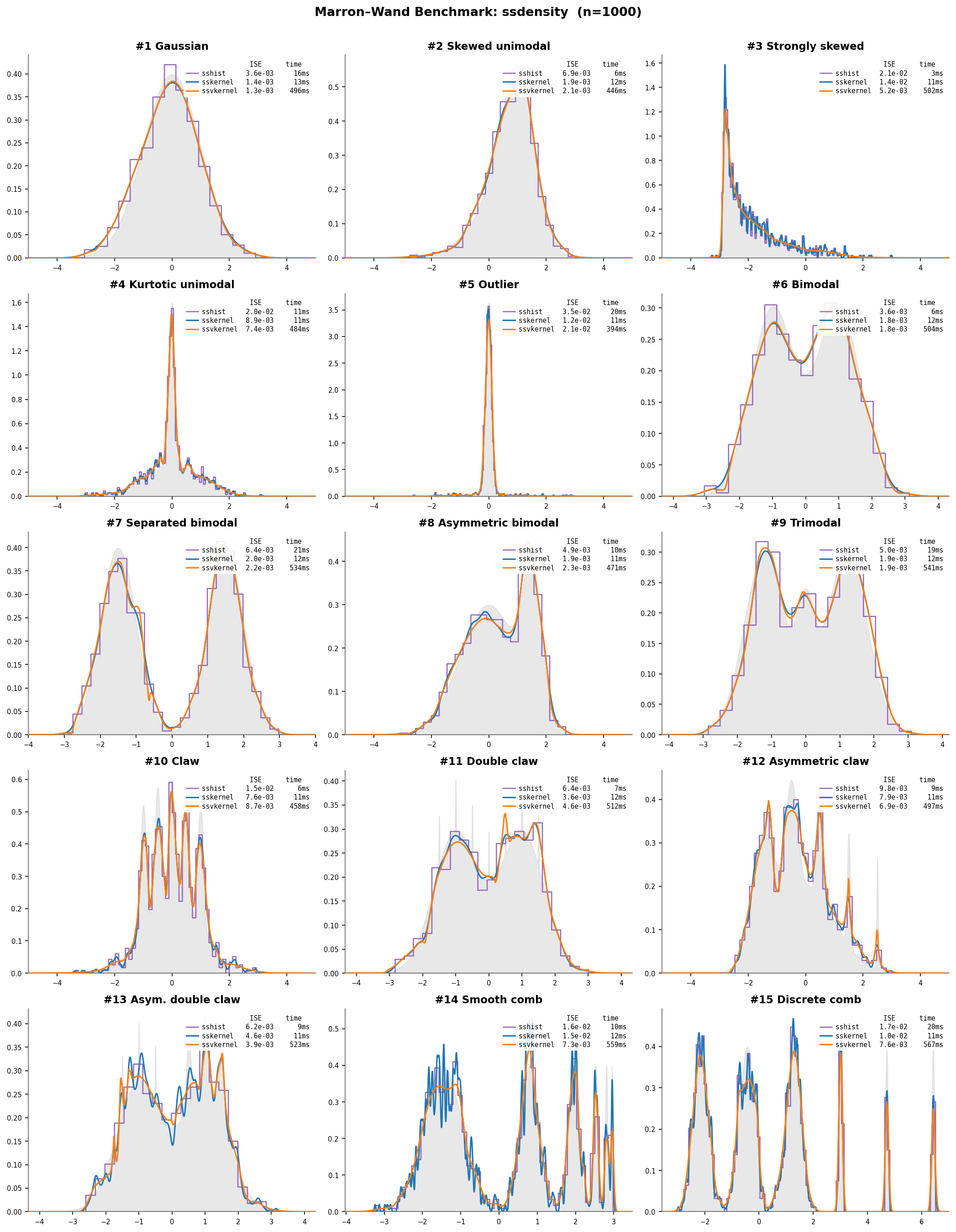
Gray fill = true density; sshist (purple), sskernel (blue),
ssvkernel (orange) ($n = 1000$). Each subplot shows ISE and wall time.
ssvkernel tracks fine structure (#10 Claw, #15 Discrete comb) that
sskernel smooths over.
J. S. Marron and M. P. Wand, "Exact mean integrated squared error," The Annals of Statistics 20(2): 712-736, 1992. doi:10.1214/aos/1176348653
Comparison of methods
Fourteen density estimation methods are evaluated on the 15 Marron-Wand (1992) benchmark densities ($n = 1000$, 50 Monte Carlo runs per density). Besides the three ssdensity methods, the comparison includes:
- KDE diffusion -- diffusion-based plug-in bandwidth (Botev et al. 2010;
kde_diffusion) - KDEpy ISJ -- Improved Sheather-Jones via diffusion (Nagler 2018;
KDEpy) - KDEpy Silverman -- Silverman rule-of-thumb (Silverman 1986;
KDEpy) - scipy kde -- Scott's rule (Scott 1992;
scipy) - statsmodels KDE -- normal-reference bandwidth (Silverman 1986;
statsmodels) - fastkde -- self-consistent field bandwidth (Bernacchia & Pigolotti 2011;
fastkde) - awkde -- adaptive-width KDE with sensitivity parameter (Cranmer 2001;
awkde) - Neural Spline Flow -- normalizing flow with rational-quadratic splines (Durkan et al. 2019;
normflows) - Zuko UNAF -- UMNN-based autoregressive flow (Wehenkel & Louppe 2019;
zuko) - ARF -- adversarial random forest density estimation (Watson et al. 2023;
arf) - TransportMap -- polynomial transport map with KL fit (Marzouk et al. 2016;
TransportMaps)
All methods use default settings for a fair comparison.
Example fits on challenging densities
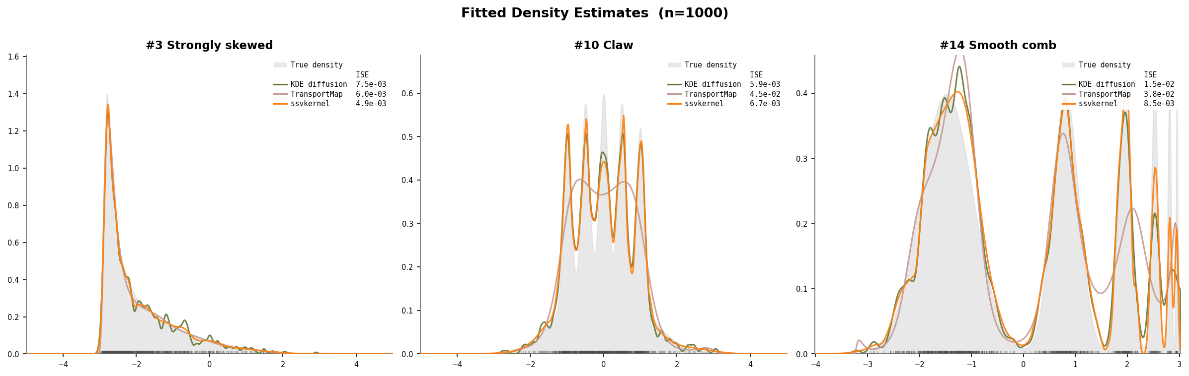
Three representative Marron–Wand densities (n=1000): #3 Strongly skewed (8 cascading components), #10 Claw (narrow spikes on a broad mode), and #14 Smooth comb (6 components at different scales). The gray fill shows the true density. ssvkernel (orange) closely tracks the true shape, while KDE diffusion slightly over-smooths the fine structure and TransportMap struggles with multi-scale detail.
Assessment of estimation error
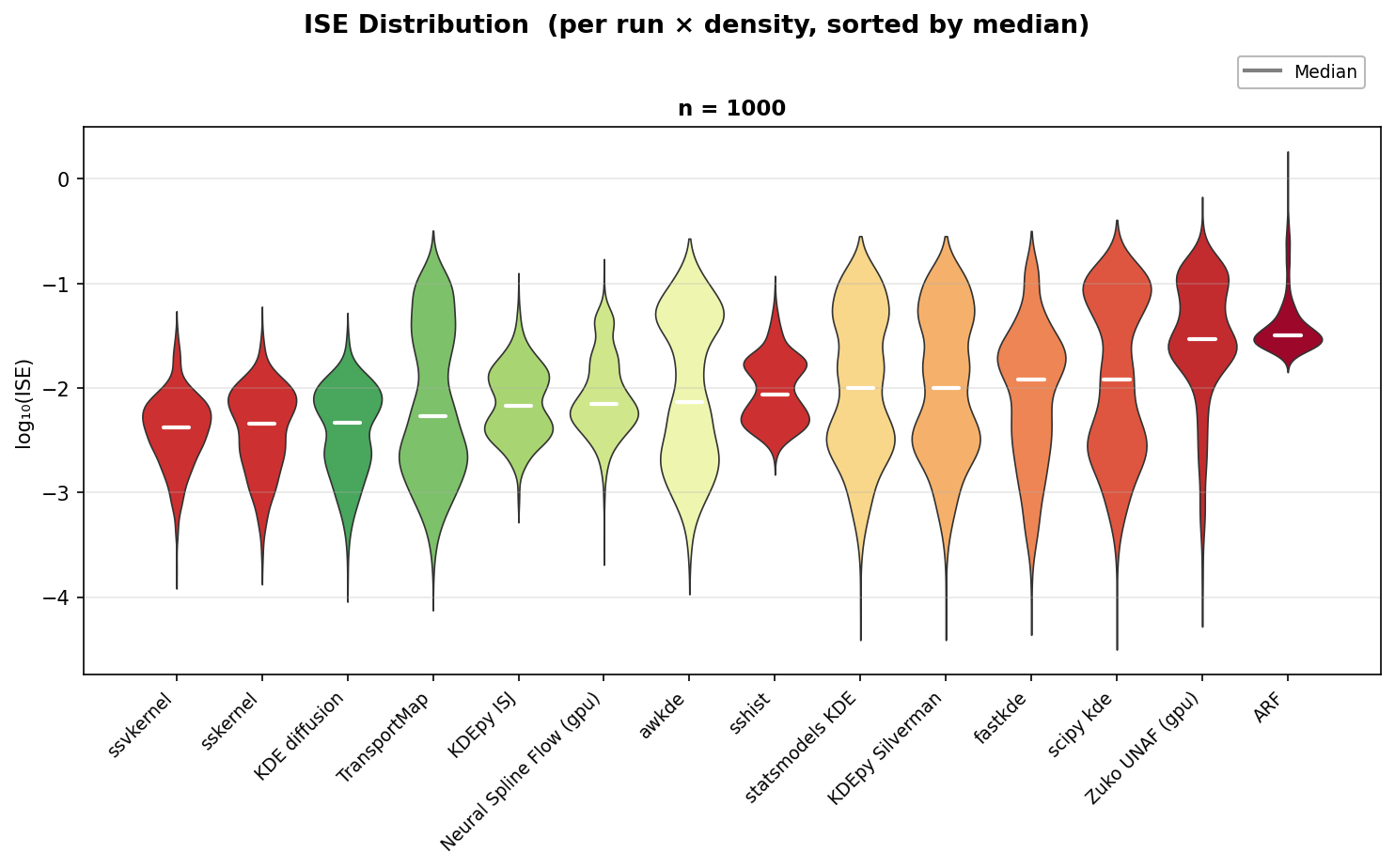
Each violin shows the distribution of Integrated Squared Error (ISE) across
all 750 (density, run) pairs on a log10 scale. Methods are sorted left to right
by median ISE (white line); lower is better.
ssvkernel, KDE diffusion, and sskernel form the top tier with the lowest
medians and tightest distributions.
Accuracy vs speed
Speed or accuracy? sskernel is both fast and accurate.
For the best accuracy on complex shapes, ssvkernel wins.
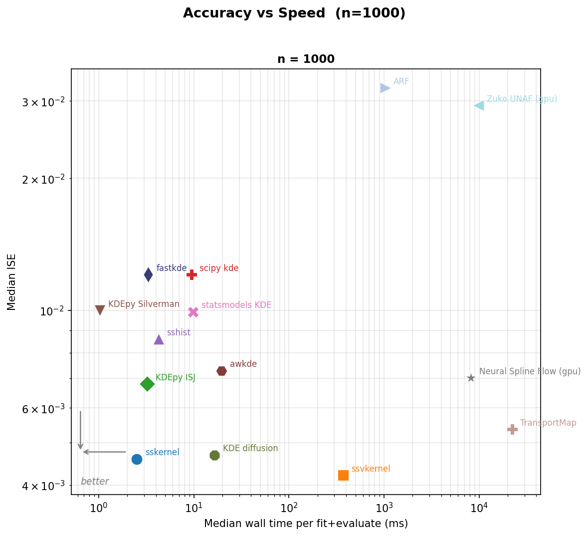
Pooled median ISE (y-axis, log scale) versus mean wall time per fit-and-evaluate call (x-axis, log scale). Points closer to the lower-left corner are both more accurate and faster.
Error by method and density
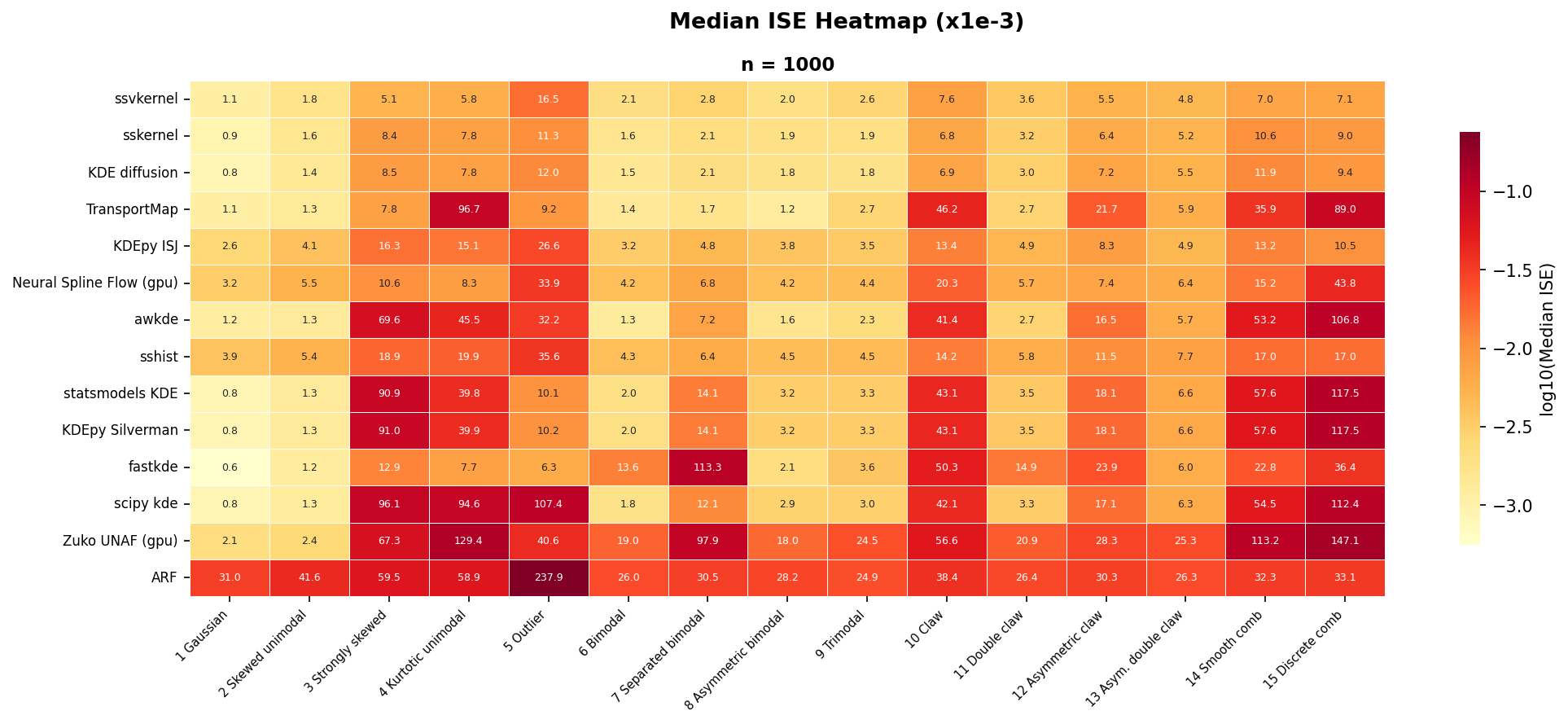
Median ISE ($\times 10^{-3}$) for each method-density pair, sorted by pooled median ISE (best at top). Darker cells indicate lower (better) error.
ssvkernel achieves the best median ISE overall and ranks first on 6 of
the 15 densities — specifically, the most challenging shapes that require
locally adaptive bandwidth: #3 Strongly skewed, #4 Kurtotic unimodal,
#12 Asymmetric claw, #13 Asymmetric double claw, #14 Smooth comb, and
#15 Discrete comb. sskernel wins #10 Claw and places in the top 3 on
12 of 15 densities. Together, the two kernel methods maintain
consistently low error across all 15 densities.
Speed improvement
Optimized from the original AdaptiveKDE (PyPI: adaptivekde). Median wall time on Marron-Wand #1 Gaussian ($n = 1000$, 3 warmup + 20 measured runs, $2\times$ Xeon 6258R / 112 threads):
| Function | Classic (ms) | Optimized (ms) | Speedup |
|---|---|---|---|
sshist |
750 | 3.0 | 248x |
sskernel |
47 | 22 | 2x |
ssvkernel |
2616 | 482 | 5x |
- sshist: Numba JIT with parallel outer loop (
prange) over candidate bin counts; replaces per-shiftnp.histogramwith vectorizedsearchsorted - sskernel: Real FFT (
rfft/irfft) halves transform size versus complex FFT; batched bootstrap FFTs in a single 2-D array call - ssvkernel: Batched FFTs grouped by padded length (~6400 individual FFTs → ~3 forward + ~80 inverse); vectorized Nadaraya–Watson kernel regression via broadcasting; vectorized bootstrap loop
Reproduce: python benchmarks/performance_comparison/run_mise_comparison.py
and python benchmarks/speed_comparison/classic_vs_optimized.py
References
-
H. Shimazaki and S. Shinomoto, "A method for selecting the bin size of a time histogram," Neural Computation 19(6): 1503-1527, 2007. doi:10.1162/neco.2007.19.6.1503
@article{shimazaki2007histogram,
  author  = {Shimazaki, Hideaki and Shinomoto, Shigeru},
  title   = {A Method for Selecting the Bin Size of a Time Histogram},
  journal = {Neural Computation},
  volume  = {19},
  number  = {6},
  pages   = {1503--1527},
  year    = {2007},
  doi     = {10.1162/neco.2007.19.6.1503}
}
-
H. Shimazaki and S. Shinomoto, "Kernel bandwidth optimization in spike rate estimation," Journal of Computational Neuroscience 29(1-2): 171-182, 2010. doi:10.1007/s10827-009-0180-4
@article{shimazaki2010kernel,
  author  = {Shimazaki, Hideaki and Shinomoto, Shigeru},
  title   = {Kernel Bandwidth Optimization in Spike Rate Estimation},
  journal = {Journal of Computational Neuroscience},
  volume  = {29},
  number  = {1--2},
  pages   = {171--182},
  year    = {2010},
  doi     = {10.1007/s10827-009-0180-4}
}
Authors
- Hideaki Shimazaki (shimazaki.hideaki.8x@kyoto-u.jp) -- shimazaki on GitHub (maintainer)
The original Python code (PyPI: adaptivekde) was created by
- Lee A.D. Cooper (cooperle@gmail.com) -- cooperlab on GitHub
- Subhasis Ray (ray.subhasis@gmail.com)
based on the MATLAB code developed by Shimazaki.
License
Apache License 2.0. See LICENSE.txt for details.
Release history Release notifications | RSS feed


Download files
Download the file for your platform. If you're not sure which to choose, learn more about installing packages.
Source Distribution
Built Distribution
Filter files by name, interpreter, ABI, and platform.
If you're not sure about the file name format, learn more about wheel file names.
Copy a direct link to the current filters
File details
Details for the file ssdensity-0.1.1.tar.gz.
File metadata
- Download URL: ssdensity-0.1.1.tar.gz
- Upload date:
- Size: 2.9 MB
- Tags: Source
- Uploaded using Trusted Publishing? No
- Uploaded via: twine/6.2.0 CPython/3.11.14
File hashes
| Algorithm | Hash digest | |
|---|---|---|
| SHA256 |
2516b53383b2fe994ffbaae9a078a9c973ae1570bc0f6c78190516a0bc99018e
|
|
| MD5 |
6530265fb6a982c2b5c138e90d5041f1
|
|
| BLAKE2b-256 |
65d6aadd1b5a87b92bf8a93ed9c506cf96d7a866168c89a25a369afd9b93e1d2
|
File details
Details for the file ssdensity-0.1.1-py3-none-any.whl.
File metadata
- Download URL: ssdensity-0.1.1-py3-none-any.whl
- Upload date:
- Size: 27.0 kB
- Tags: Python 3
- Uploaded using Trusted Publishing? No
- Uploaded via: twine/6.2.0 CPython/3.11.14
File hashes
| Algorithm | Hash digest | |
|---|---|---|
| SHA256 |
15bb1a8ae78481295a8e235941bed16000b39e7afa0bffbd0837347866171c9f
|
|
| MD5 |
89b6e316661fac0b29966781ba5a0441
|
|
| BLAKE2b-256 |
eaf26aea182a792ed51d409b28b9773fa48d473515be6d30f4fa20ae2d045c69
|


