
Wandas is an open source library for efficient signal analysis in Python

Project description
Wandas
English | 日本語






Signal analysis that feels like working with a data frame.
Wandas is a Python library for treating audio, vibration, sensor, and other waveform data as a ChannelFrame. Samples stay together with their sampling rate, channel names, units, metadata, and processing history as you read, preprocess, analyze, and visualize a signal.
Signal-analysis code often keeps the waveform in a NumPy array, the sampling rate in another variable, labels and units in a dictionary, and processing notes in notebook comments. Wandas gathers that context into one frame, so the intent reads directly in code: wd.read(...) → remove_dc() → low_pass_filter() → fft() → plot().
Methods do not mutate their input; each one returns a new frame. The result records operation_history, and previous points back to the preceding frame, making before-and-after checks easy. This reviewable workflow helps when you review the analysis as a team or ask an AI agent to check it: the code, data context, processing history, and figures remain connected.
Why Wandas
-
The processing flow reads naturally
Traditional workflows connect NumPy, SciPy, Matplotlib, and other libraries while repeatedly checking array shapes and axes. Wandas exposes reading, filtering, FFT, and visualization as frame methods in the order you use them.
-
The frame carries data context and processing history
Sampling rate, channel names, units, and metadata stay with the waveform.
operation_historyandpreviouslet you trace which operation produced each result. -
Visualization is close at hand
Signal analysis works best when you can inspect waveforms, spectra, and spectrograms alongside the numbers.
describe()shows the main views together, and each frame providesplot()for quick visualization. -
Real-world inputs enter the same workflow
WAV, FLAC, OGG, AIFF, SND, CSV, URLs, bytes, file-like objects, and NumPy arrays all feed into the same frame-based API. Once loaded, recordings and sensor data follow the same analysis flow.
-
The workflow scales toward larger data and ML preprocessing
Frame processing is Dask-backed and lazy by default, while
ChannelFrameDatasetlazily loads multiple files from a folder. You can chain resampling, trimming, normalization, and STFT before converting results to PyTorch or TensorFlow tensors when needed.
Installation
For the best first experience, install the extra that includes interactive display support and the marimo learning app:
pip install "wandas[marimo]"
If you already use Jupyter or IPython, or only need to save figures to files, you can start with the core package:
pip install wandas
The core package includes waveform frames, CSV/WAV reading, signal processing, Matplotlib plots, and describe() figure creation and export through options such as is_close=False and image_save.
Combine optional extras as needed:
pip install "wandas[io]"              # WDF save and load
pip install "wandas[effects]"         # librosa-backed audio effects
pip install "wandas[marimo]"          # marimo learning app and interactive display
pip install "wandas[psychoacoustic]"  # loudness, roughness, sharpness, and related metrics
pip install "wandas[ml]"              # PyTorch / TensorFlow tensor conversion

pip install "wandas[marimo,io,effects,psychoacoustic]"
Inspect the Sample Audio
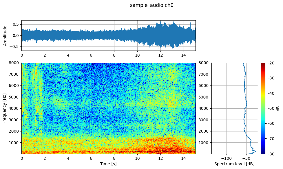
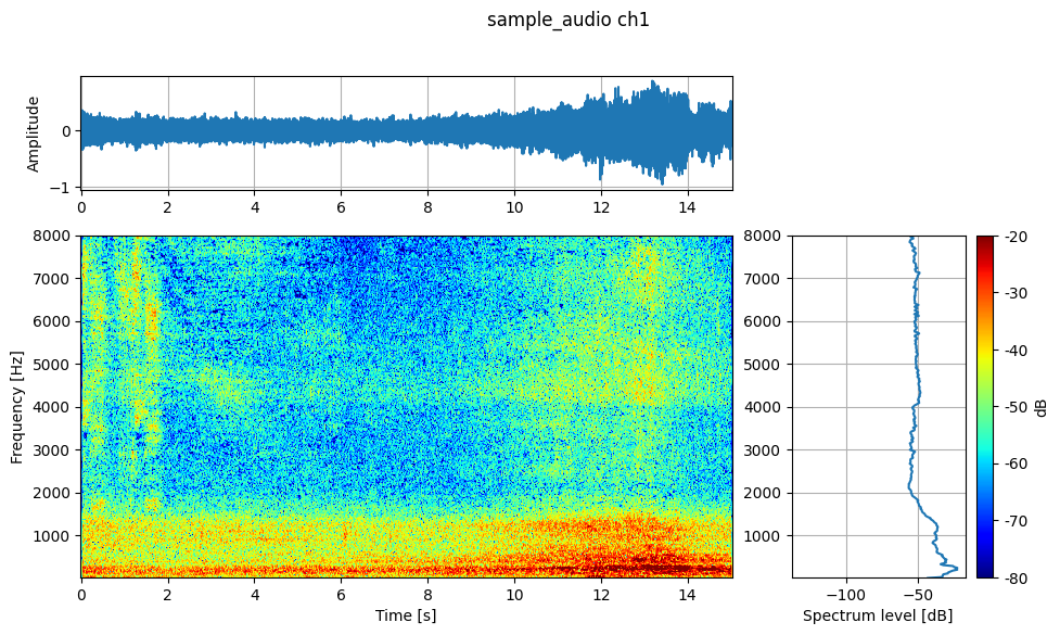
Start with describe() to see the recording as a whole. The example uses the bundled file in a repository checkout and the same sample's public URL in an installed environment, so you can run it as written in either case.
from pathlib import Path

import wandas as wd

local_sample = Path("learning-path/sample_audio.wav")
sample_source = (
    local_sample
    if local_sample.exists()
    else "https://raw.githubusercontent.com/kasahart/wandas/main/learning-path/sample_audio.wav"
)

recording = wd.read(sample_source, end=15)
recording.describe(fmin=20, fmax=8_000, vmin=-80, vmax=-20, image_save="readme_sample_audio_describe.png")
Before you decide what to clean or measure, describe() presents the waveform, spectrogram, and Welch spectrum together. For a multichannel frame, it saves one figure per channel.
The workflow stays method-centered from here. Call recording.remove_dc() to remove a DC offset, .low_pass_filter(cutoff=1_000) to apply a low-pass filter, .fft() to move into the frequency domain, and .plot() on the result to visualize it. You do not need to pass the array, sampling rate, and channel context through separate helper variables.
frame.normalize()transforms the frame data. In contrast,frame.describe(normalize=True)normalizes only playback and leaves the analyzed data unchanged.wd.read()has nonormalizeargument. Use data converted to Pa for SPL and psychoacoustic metrics that require calibrated values.
Validate with a Known Signal
Next, verify that the code and analysis result agree for a signal whose answer is known. wd.from_numpy() creates a ChannelFrame from a NumPy array while attaching the sampling rate, channel names, and units.
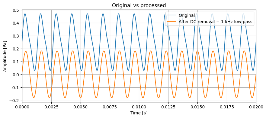
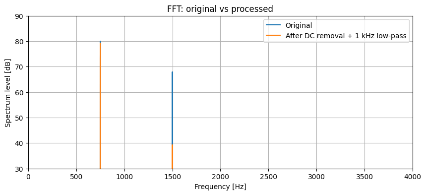
This example creates one mono signal containing 750 Hz and 1500 Hz tones plus a DC offset. It removes DC, applies a 1 kHz low-pass filter in one method chain, and combines the result with the original through add_channel() for overlaid waveform and FFT views.
import numpy as np
import wandas as wd

sr = 48_000
t = np.arange(sr) / sr


def tone(components, *, offset=0.0):
    return offset + sum(amplitude * np.sin(2 * np.pi * freq * t) for freq, amplitude in components)


samples = tone([(750, 0.20), (1500, 0.05)], offset=0.25).astype(np.float64)

signal = wd.from_numpy(
    samples,
    sampling_rate=sr,
    label="known signal",
    ch_labels=["Original"],
    ch_units="Pa",
)

processed = (
    signal
    .remove_dc()
    .low_pass_filter(cutoff=1_000)
    .rename_channels({0: "After DC removal + 1 kHz low-pass"})
)
comparison = signal.add_channel(processed)

comparison.plot(
    overlay=True,
    xlim=(0, 0.02),
    title="Original vs processed",
)
spectrum_ax = comparison.fft().plot(
    overlay=True,
    xlim=(0, 4_000),
    title="FFT: original vs processed",
)
spectrum_ax.set_ylim(30, 90)
The method chain returns a new ChannelFrame without changing the original signal. processed.previous follows the preceding frame, while processed.operation_history records both remove_dc() and low_pass_filter().
signal.add_channel(processed) combines the original and processed signals into a two-channel comparison frame. In the waveform overlay, the DC offset disappears and the filtered waveform changes shape.
The FFT overlay uses a fixed 30–90 dB vertical range. It shows that the processed signal keeps the 750 Hz component while attenuating the 1500 Hz component above the 1 kHz cutoff.
Use Your Own Data
After confirming the workflow with the sample, replace the input with your own WAV or CSV file. The same frame-first API carries you from reading through preprocessing, visualization, and frequency analysis.
import wandas as wd

recording = wd.read("recording.wav", end=15)
clean = recording.remove_dc().normalize()
spectrum = clean.welch()
fmax = min(8_000, clean.sampling_rate / 2)

clean.describe(fmin=20, fmax=fmax, vmin=-80, vmax=-20, image_save="recording_overview.png")
spectrum.plot(xlim=(20, fmax))
Preserve calibration when analyzing physical quantities. Because normalize() changes amplitude, calculate SPL, sound level, loudness, roughness, sharpness, and similar metrics from the original data after correctly converting it to Pa. Read the calibrated NumPy values from frame.data; the internal array backend does not need to be managed directly. The executable per-channel calibration learning path covers certificate and CSV-managed factors, acceleration, 100-channel configuration, and WDF round-trips. Psychoacoustic metrics require wandas[psychoacoustic], while WDF save and load require wandas[io].
For multiple files, start with wd.from_folder("recordings/", recursive=True). Apply preprocessing to the dataset with a chain such as .resample(16_000).trim(0, 5).normalize().stft(n_fft=512). To pass a frame to ML code, use frame.to_tensor(framework="torch") or frame.to_tensor(framework="tensorflow") (wandas[ml] is required, and conversion materializes the lazy data).
Select files before reading waveforms
When folders describe groups or recording batches, let Wandas infer that metadata during discovery and select only the files you need:
Create the dataset with dataset = wd.from_folder("recordings/", recursive=True, path_metadata=True), then select a group with selected = dataset.select(partition_0="group_a").
Plain folders become partition_0, partition_1, and so on; Hive-style folders such as group=group_a use group as the key. File selection does not read audio headers or waveform samples. Use metadata_resolver only when metadata must come from custom filename rules or an external table. The executable metadata-driven dataset search learning path covers the recommended folder workflow, CSV lookup, lazy loading, and dataset-wide processing before selection.
Small top-level API
wd.read("audio.wav"): read WAV, CSV, supported audio, URL, bytes, or file-like input into aChannelFrame.wd.from_numpy(data, sampling_rate=48_000): create a frame from a NumPy array.wd.from_folder("recordings/", recursive=True): create a lazy folder-backed dataset.wd.load("analysis.wdf"): load Wandas native WDF withwandas[io].wd.supported_formats(): inspect registered reader formats.
Read WDF with wd.load(), not wd.read(). read_wav(), read_csv(), and from_ndarray() remain available for existing code, but new examples use read() and from_numpy().
Core Objects
ChannelFrame: multichannel waveform or sensor data in the time domain.SpectralFrame: FFT, Welch, coherence, CSD, and transfer-function results.SpectrogramFrame: STFT and other time-frequency data.NOctFrame: octave and fractional-octave spectra.ChannelFrameDataset: a lazy collection for loading and preprocessing recordings from a folder.
Good Fits
Wandas is especially useful when you want to:
- prototype a signal-processing pipeline while inspecting waveforms in a notebook or marimo;
- preserve labels, units, and processing history for audio, vibration, or sensor data;
- compare multiple WAV or CSV files through the same preprocessing and analysis API;
- review signal-processing steps and results with teammates or AI agents;
- build STFT and related features before PyTorch or TensorFlow preprocessing.
Learn More
- Documentation - Guides, API reference, and examples.
- Learning Path - Step-by-step marimo learning apps.
- Tutorial - A guided walkthrough of the core workflow.
- Issue Tracker - Report bugs or propose ideas.
Project Status
Wandas is actively evolving. The package targets Python 3.10+ and is published under the MIT License. For production workflows, pin the version and review the release notes before upgrading.
Contributing
Contributions are welcome.
For development setup, quality checks, documentation conventions, and the pull request workflow, see docs/src/contributing.md.
License
Released under the MIT License.
Release history Release notifications | RSS feed


Download files
Download the file for your platform. If you're not sure which to choose, learn more about installing packages.
Source Distribution
Built Distribution
Filter files by name, interpreter, ABI, and platform.
If you're not sure about the file name format, learn more about wheel file names.
Copy a direct link to the current filters
File details
Details for the file wandas-0.6.0.tar.gz.
File metadata
- Download URL: wandas-0.6.0.tar.gz
- Upload date:
- Size: 7.9 MB
- Tags: Source
- Uploaded using Trusted Publishing? No
- Uploaded via: twine/6.1.0 CPython/3.13.14
File hashes
| Algorithm | Hash digest | |
|---|---|---|
| SHA256 |
702cfd2db225cb8b1918b82a6c3e8b79efe0ae4ea2cdf18cf4ae463fa420cf05
|
|
| MD5 |
ce95b48cc9d8106bdd3a506c9b20b25e
|
|
| BLAKE2b-256 |
a25600119fbec041878778e35a44085c084254e6402a09eb1edb87925a48185c
|
File details
Details for the file wandas-0.6.0-py3-none-any.whl.
File metadata
- Download URL: wandas-0.6.0-py3-none-any.whl
- Upload date:
- Size: 216.2 kB
- Tags: Python 3
- Uploaded using Trusted Publishing? No
- Uploaded via: twine/6.1.0 CPython/3.13.14
File hashes
| Algorithm | Hash digest | |
|---|---|---|
| SHA256 |
4edd2044037510caea3bcd7476a3a0fdf24ffd9cca588319b5719b6852a311e8
|
|
| MD5 |
3b23f305e4f5e60ddb860f5988983544
|
|
| BLAKE2b-256 |
2b32fffc1bdad0f4d1b6157a8961151605b91a6d5209309fa7133cfb70d24695
|






