
RiskOptima





RiskOptima is a comprehensive Python toolkit for evaluating, managing, and optimizing investment portfolios. This package is designed to empower investors and data scientists by combining financial risk analysis, backtesting, mean-variance optimization, and machine learning capabilities into a single, cohesive package.
Stats
https://pypistats.org/packages/riskoptima
Key Features
- Modular Core:
MarketData,Portfolio, andBacktestConfigtypes for clean workflows. - Backtesting Framework: Strategy interfaces, cost/slippage modeling, and performance tracking.
- Risk Models: Factor risk model with exposures and factor-based covariance estimation.
- Optimization: Mean-variance, efficient frontier, max Sharpe, and constraint handling (bounds, leverage, turnover, factor limits).
- Risk Management: VaR, CVaR, volatility, and drawdown analytics.
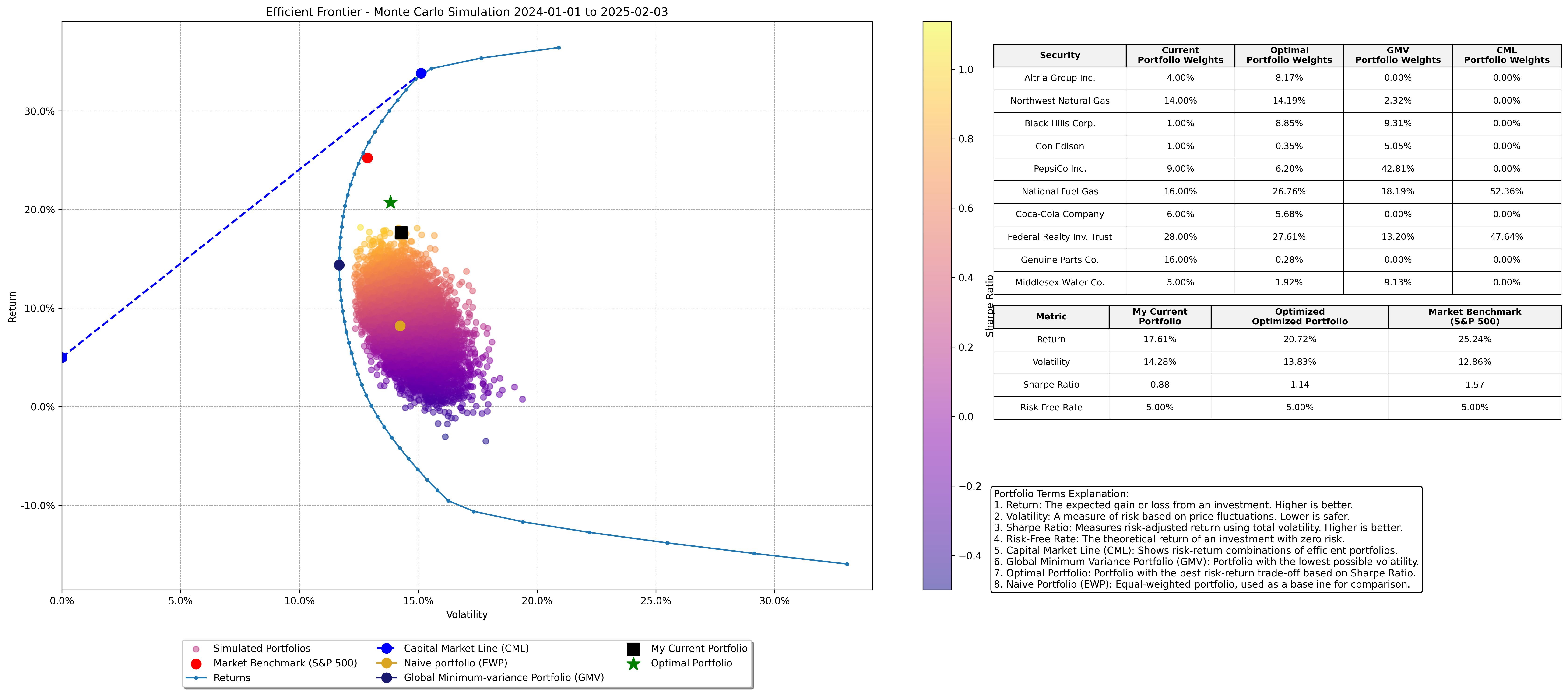
- Monte Carlo Simulations: Analyze potential portfolio outcomes. See example here https://github.com/JordiCorbilla/efficient-frontier-monte-carlo-portfolio-optimization
- Market & Allocation Visuals: Correlation matrices, portfolio area charts, and diagnostics.
- Quant Models: Black-Litterman, stochastic volatility models, and options/Greeks analytics.
- Portfolio Projects: algorithmic trading/backtesting, portfolio optimization, market risk dashboard, option pricing engine, and credit risk model workflows.
Quant Portfolio Project Map
| Project | Notebook / Example | Package API | Screenshot |
|---|---|---|---|
| Algorithmic Trading Backtester | 05-portfolio_sma_strategy.ipynb |
riskoptima.backtest |
 |
| Portfolio Optimization | 02-portfolio_optimization_riskoptima.ipynb |
riskoptima.optim |
 |
| Market Risk Dashboard | examples/example_market_risk_dashboard.py |
riskoptima.reporting |
 |
| Option Pricing Engine | examples/example_option_pricing_engine.py |
riskoptima.options |
 |
| Credit Risk Model | 08-credit_risk_model_demo.ipynb |
riskoptima.credit |
 |
See docs/quant_project_map.md for a recruiter/interviewer-friendly walkthrough of the five projects.
Installation
See the project here: https://pypi.org/project/riskoptima/
pip install riskoptima
Usage
New modular API (backtest + factor risk + constraints)
import pandas as pd
from riskoptima import FactorRiskModel, Constraints, optimize_max_sharpe
from riskoptima import SMACrossStrategy, run_backtest, BacktestConfig, SimpleCostModel

# prices: DataFrame with Date index and asset columns
prices = pd.read_csv("prices.csv", index_col=0, parse_dates=True)
asset_returns = prices.pct_change().dropna()

# factors: Fama-French returns DataFrame (e.g. from RiskOptima.get_fff_returns)
factors = pd.read_csv("fama_french_factors.csv", index_col=0, parse_dates=True)

factor_model = FactorRiskModel(factor_returns=factors).fit(asset_returns)
factor_cov = factor_model.covariance_matrix()

constraints = Constraints(factor_bounds={"MKT": (-0.2, 0.8)})
weights = optimize_max_sharpe(
    expected_returns=asset_returns.mean() * 252,
    cov=factor_cov,
    constraints=constraints,
    factor_exposures=factor_model.exposures,
    risk_free_rate=0.02,
)

strategy = SMACrossStrategy(short_window=20, long_window=50)
config = BacktestConfig(initial_cash=1_000_000, rebalance_rule="D")
cost_model = SimpleCostModel(spread_bps=2.0, impact_coeff=0.0)
equity_curve, weights_history = run_backtest(prices, strategy, config, cost_model)
See examples/example_factor_backtest.py for a runnable end-to-end example.
SMA Crossover Strategy
RiskOptima includes reusable SMA crossover helpers for a simple long-only trend-following workflow. The short moving average crossing above the long moving average creates an entry signal; a bearish cross, stop loss, or take profit closes the trade.
from riskoptima.backtest import build_sma_signal_frame, run_sma_strategy_with_risk

signals = build_sma_signal_frame(prices[["Close"]], short_window=20, long_window=50)
trades = run_sma_strategy_with_risk(
    "SPY",
    start="2024-01-01",
    end="2025-01-01",
    stop_loss=0.05,
    take_profit=0.10,
)
The notebook 05-portfolio_sma_strategy.ipynb shows single-asset, equal-weight multi-asset, and custom-weight portfolio runs.
Offline sample datasets
RiskOptima includes small synthetic datasets for deterministic examples:
data/synthetic_market_returns.csvdata/synthetic_credit_portfolio.csv
These are intentionally small and have no external data dependency.
Credit Risk Model
RiskOptima includes a production-ready credit risk layer for PD/LGD/EAD portfolios, expected loss, unexpected loss, rating migration, Merton structural default probability, and Credit VaR/CVaR Monte Carlo.
import pandas as pd
from riskoptima.credit import (
    expected_loss,
    portfolio_expected_loss,
    simulate_credit_losses,
    credit_var,
    credit_cvar,
    merton_pd,
)

portfolio = pd.DataFrame({
    "obligor": ["A", "B", "C"],
    "PD": [0.01, 0.025, 0.04],
    "LGD": [0.40, 0.45, 0.55],
    "EAD": [1_000_000, 750_000, 500_000],
})

print(expected_loss(0.02, 0.45, 1_000_000))
print(portfolio_expected_loss(portfolio))

losses = simulate_credit_losses(portfolio, n_sims=20_000, random_state=42)
print(credit_var(losses, confidence=0.99))
print(credit_cvar(losses, confidence=0.99))
print(merton_pd(asset_value=150, debt_face_value=100, asset_vol=0.25, risk_free_rate=0.03, maturity=1.0))
See 08-credit_risk_model_demo.ipynb for an end-to-end notebook.
Market Risk Dashboard
RiskOptima can build a dashboard-ready market risk report with annualized return, volatility, Sharpe, Sortino, drawdown, historical VaR, Gaussian VaR, CVaR/expected shortfall, beta, tracking error, information ratio, rolling volatility, and rolling drawdown.
Screenshot placeholder: plots/market_risk_dashboard.png
import pandas as pd
from riskoptima.reporting import build_market_risk_report

returns = pd.DataFrame({
    "AssetA": [0.01, -0.005, 0.004, 0.002],
    "AssetB": [0.002, 0.003, -0.006, 0.005],
})
weights = pd.Series({"AssetA": 0.6, "AssetB": 0.4})

report = build_market_risk_report(returns, weights=weights, confidence_levels=(0.95, 0.99))
print(report.metrics["annualized_volatility"])
print(report.metrics["historical_var"][0.99])
Run examples/example_market_risk_dashboard.py to generate a multi-panel dashboard.
Optional Streamlit dashboard:
pip install streamlit
streamlit run examples/streamlit_market_risk_dashboard.py
Option Pricing Engine
The clean options API covers Black-Scholes call/put pricing, Greeks, implied volatility, binomial trees, and Monte Carlo European option pricing while preserving the legacy RiskOptima class methods.
import pandas as pd
from riskoptima.options import (
    black_scholes_price,
    black_scholes_greeks,
    implied_volatility,
    monte_carlo_european_option,
)

S, K, T, r, sigma = 100, 100, 1.0, 0.05, 0.20
call = black_scholes_price(S, K, T, r, sigma, option_type="call")
put = black_scholes_price(S, K, T, r, sigma, option_type="put")
greeks = pd.Series(black_scholes_greeks(S, K, T, r, sigma, option_type="call"))
iv = implied_volatility(call, S, K, T, r, option_type="call")
mc = monte_carlo_european_option(S, K, T, r, sigma, option_type="call", random_state=42)

print(call, put)
print(greeks)
print(iv, mc)
Run examples/example_option_pricing_engine.py for a full pricing comparison.
Example 1: Setting up your portfolio
Create your portfolio table similar to the below:
| Asset | Weight | Label | MarketCap |
|---|---|---|---|
| MO | 0.04 | Altria Group Inc. | 110.0e9 |
| NWN | 0.14 | Northwest Natural Gas | 1.8e9 |
| BKH | 0.01 | Black Hills Corp. | 4.5e9 |
| ED | 0.01 | Con Edison | 30.0e9 |
| PEP | 0.09 | PepsiCo Inc. | 255.0e9 |
| NFG | 0.16 | National Fuel Gas | 5.6e9 |
| KO | 0.06 | Coca-Cola Company | 275.0e9 |
| FRT | 0.28 | Federal Realty Inv. Trust | 9.8e9 |
| GPC | 0.16 | Genuine Parts Co. | 25.3e9 |
| MSEX | 0.05 | Middlesex Water Co. | 2.4e9 |
import pandas as pd
from riskoptima import RiskOptima

import warnings
warnings.filterwarnings(
    "ignore",
    category=FutureWarning,
    message=".*DataFrame.std with axis=None is deprecated.*"
)

# Define your current porfolio with your weights and company names
asset_data = [
    {"Asset": "MO",    "Weight": 0.04, "Label": "Altria Group Inc.",       "MarketCap": 110.0e9},
    {"Asset": "NWN",   "Weight": 0.14, "Label": "Northwest Natural Gas",   "MarketCap": 1.8e9},
    {"Asset": "BKH",   "Weight": 0.01, "Label": "Black Hills Corp.",         "MarketCap": 4.5e9},
    {"Asset": "ED",    "Weight": 0.01, "Label": "Con Edison",                "MarketCap": 30.0e9},
    {"Asset": "PEP",   "Weight": 0.09, "Label": "PepsiCo Inc.",              "MarketCap": 255.0e9},
    {"Asset": "NFG",   "Weight": 0.16, "Label": "National Fuel Gas",         "MarketCap": 5.6e9},
    {"Asset": "KO",    "Weight": 0.06, "Label": "Coca-Cola Company",         "MarketCap": 275.0e9},
    {"Asset": "FRT",   "Weight": 0.28, "Label": "Federal Realty Inv. Trust", "MarketCap": 9.8e9},
    {"Asset": "GPC",   "Weight": 0.16, "Label": "Genuine Parts Co.",         "MarketCap": 25.3e9},
    {"Asset": "MSEX",  "Weight": 0.05, "Label": "Middlesex Water Co.",       "MarketCap": 2.4e9}
]
asset_table = pd.DataFrame(asset_data)

capital = 100_000

asset_table['Portfolio'] = asset_table['Weight'] * capital

ANALYSIS_START_DATE = RiskOptima.get_previous_year_date(RiskOptima.get_previous_working_day(), 1)
ANALYSIS_END_DATE   = RiskOptima.get_previous_working_day()
BENCHMARK_INDEX     = 'SPY'
RISK_FREE_RATE      = 0.05
NUMBER_OF_WEIGHTS   = 10_000
NUMBER_OF_MC_RUNS   = 1_000
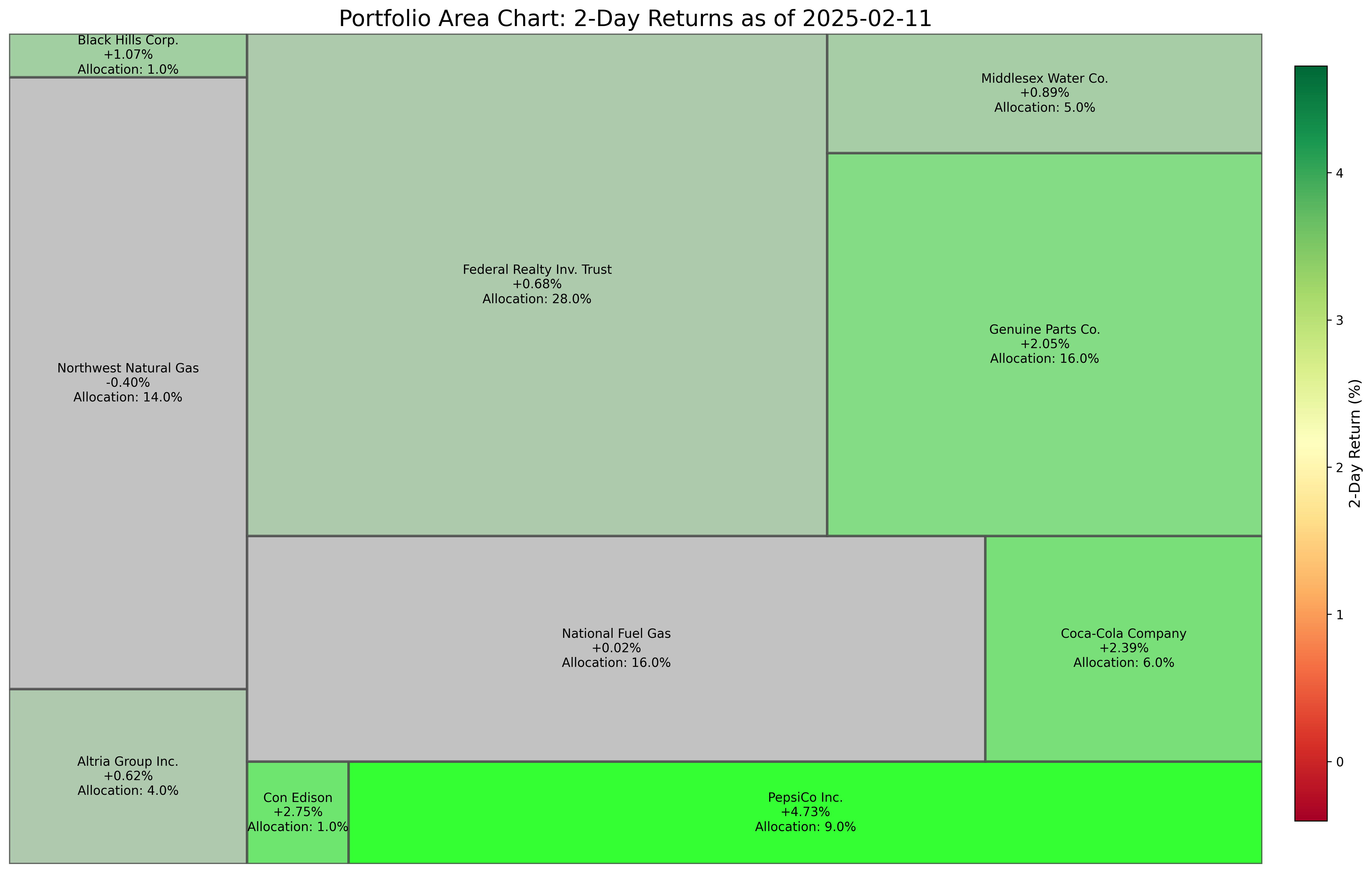
Example 1: Creating a Portfolio Area Chart
If you want to know visually how's your portfolio doing right now
RiskOptima.create_portfolio_area_chart(
    asset_table,
    end_date=ANALYSIS_END_DATE,
    lookback_days=2,
    title="Portfolio Area Chart"
)
Example 2: Efficient Frontier - Monte Carlo Portfolio Optimization
RiskOptima.plot_efficient_frontier_monte_carlo(
    asset_table,
    start_date=ANALYSIS_START_DATE,
    end_date=ANALYSIS_END_DATE,
    risk_free_rate=RISK_FREE_RATE,
    num_portfolios=NUMBER_OF_WEIGHTS,
    market_benchmark=BENCHMARK_INDEX,
    set_ticks=False,
    x_pos_table=1.15,    # Position for the weight table on the plot
    y_pos_table=0.52,    # Position for the weight table on the plot
    title=f'Efficient Frontier - Monte Carlo Simulation {ANALYSIS_START_DATE} to {ANALYSIS_END_DATE}'
)
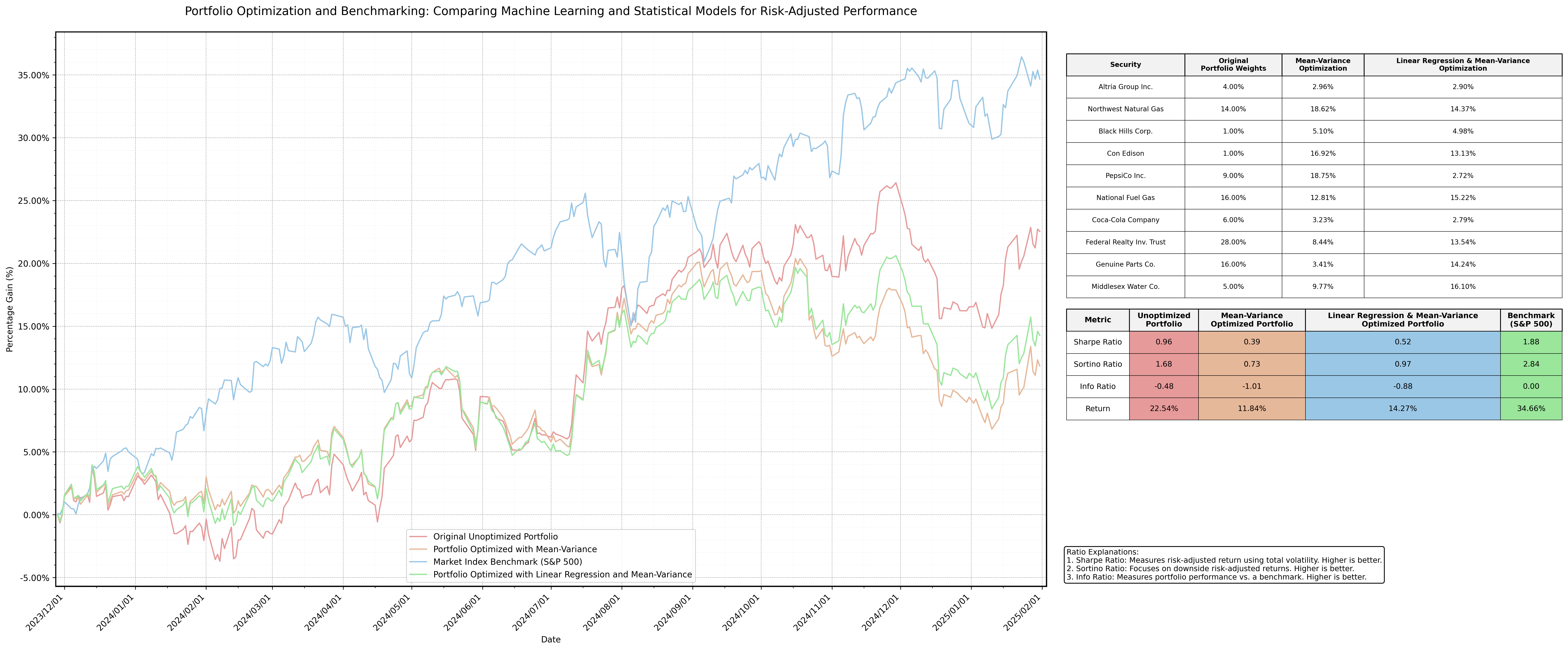
Example 3: Portfolio Optimization using Mean Variance and Machine Learning
RiskOptima.run_portfolio_optimization_mv_ml(
    asset_table=asset_table,
    training_start_date='2022-01-01',
    training_end_date='2023-11-27',
    model_type='Linear Regression',
    risk_free_rate=RISK_FREE_RATE,
    num_portfolios=100000,
    market_benchmark=[BENCHMARK_INDEX],
    max_volatility=0.25,
    min_weight=0.03,
    max_weight=0.2
)
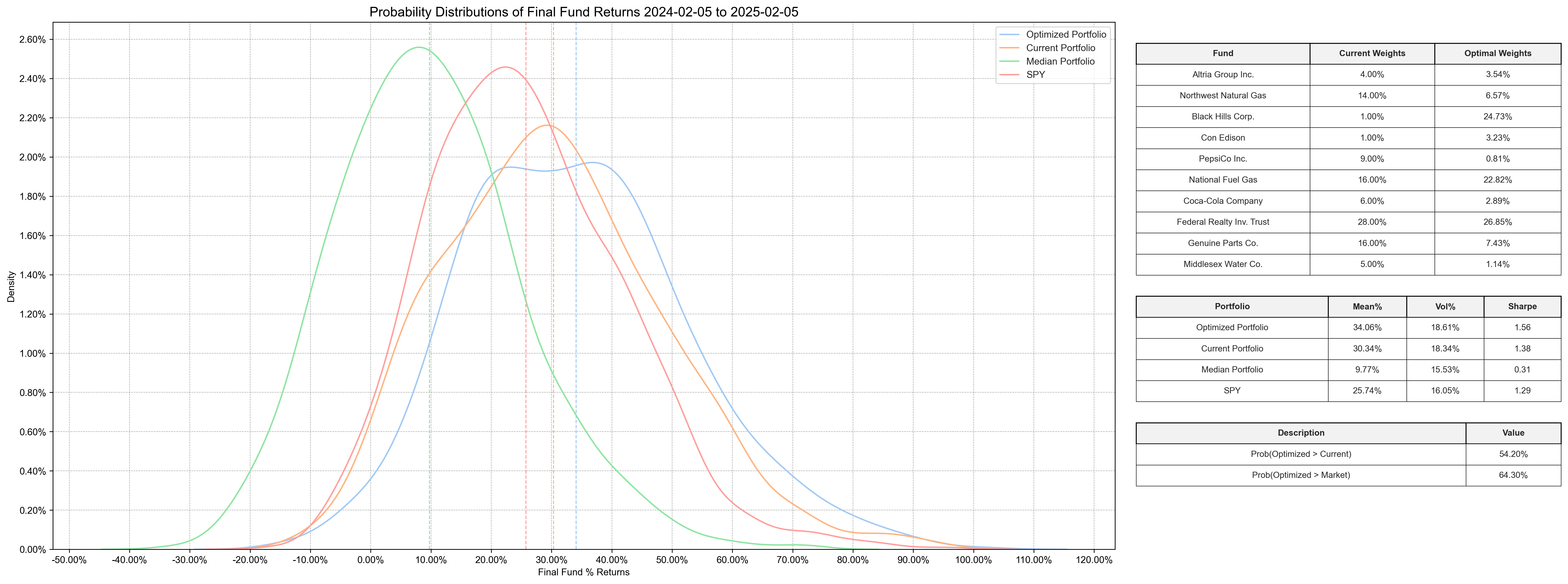
Example 4: Portfolio Optimization using Probability Analysis
RiskOptima.run_portfolio_probability_analysis(
    asset_table=asset_table,
    analysis_start_date=ANALYSIS_START_DATE,
    analysis_end_date=ANALYSIS_END_DATE,
    benchmark_index=BENCHMARK_INDEX,
    risk_free_rate=RISK_FREE_RATE,
    number_of_portfolio_weights=NUMBER_OF_WEIGHTS,
    trading_days_per_year=RiskOptima.get_trading_days(),
    number_of_monte_carlo_runs=NUMBER_OF_MC_RUNS
)
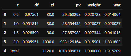
Example 5: Macaulay Duration
from riskoptima import RiskOptima
cf = RiskOptima.bond_cash_flows_v2(4, 1000, 0.06, 2)  # 2 years, semi-annual, hence 4 periods
md_2 = RiskOptima.macaulay_duration_v3(cf, 0.05, 2)
md_2
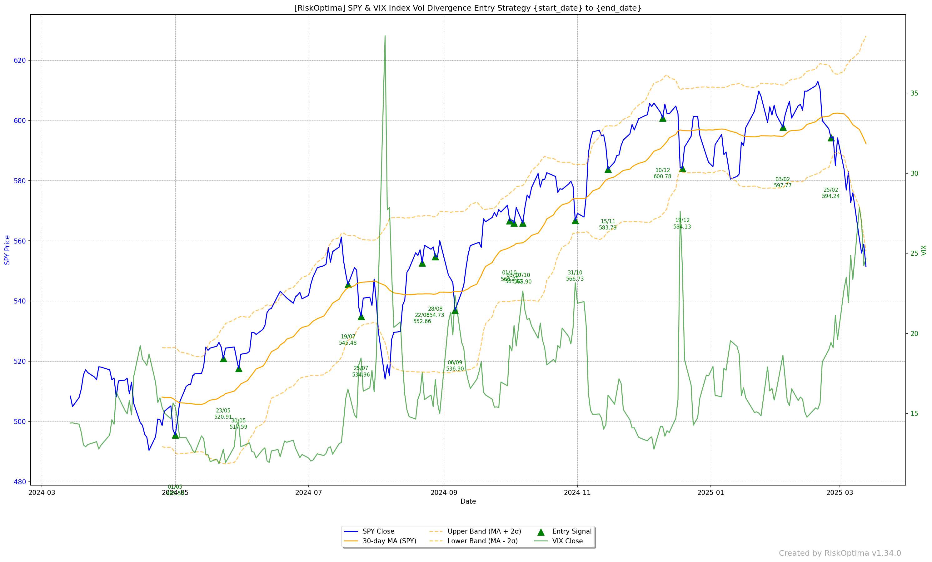
Example 6: Market Turns with SPY & VIX Divergence
ANALYSIS_START_DATE = RiskOptima.get_previous_year_date(RiskOptima.get_previous_working_day(), 1)
ANALYSIS_END_DATE   = RiskOptima.get_previous_working_day()

df_signals, df_exits, returns = RiskOptima.run_index_vol_divergence_signals(start_date=ANALYSIS_START_DATE,
                                                                            end_date=ANALYSIS_END_DATE)
Documentation
For complete documentation and usage examples, visit the GitHub repository:
Contributing
We welcome contributions! If you'd like to improve the package or report issues, please visit the GitHub repository.
License
RiskOptima is licensed under the MIT License.
Support me

1 maintainer

Metadata
1 maintainer
Release files for riskoptima 2.3.5
For a detailed explanation of source distributions (sdists) and built distributions (wheels), please see the package formats documentation.
Source distribution (sdist)
| File | Size | Uploaded | |
|---|---|---|---|
| riskoptima-2.3.5.tar.gz | 62.2 kB | Details |
Built distribution (wheel)
| File | Interpreter | ABI | Platform | Reset |
|---|---|---|---|---|
| riskoptima-2.3.5-py3-none-any.whl | Python 3 | none | any | Details |
Total release size: 130.0 kB
Release files / riskoptima-2.3.5.tar.gz
| Download URL | riskoptima-2.3.5.tar.gz |
|---|---|
| Size | 62.2 kB |
| Tags | Source |
|
SHA-256 checksum How to use checksums |
4319d87014767f21af51c9aa6926ff01d9c4aaf794e43c4907202d6ca7112cf6
|
|
BLAKE2b-256 checksum How to use checksums |
b3a0bbd5760e921d631772656f8f125132d54297e4175a141aa5659e059513d2
|
| Upload date | |
|
Uploaded using Trusted Publishing? What is trusted publishing? |
No |
| Uploaded via |
poetry/1.8.5 CPython/3.12.7 Windows/11
|
Release files / riskoptima-2.3.5-py3-none-any.whl
| Download URL | riskoptima-2.3.5-py3-none-any.whl |
|---|---|
| Size | 67.8 kB |
| Tags | Python 3 |
|
SHA-256 checksum How to use checksums |
a2fd822da238dc915cbfd82bdd2b9380a9250f8ab6688a910d929c20e40399d2
|
|
BLAKE2b-256 checksum How to use checksums |
071591ec659a96e3ecc6204f7868d6c27e54f80ce391a46898c88dd7783e844d
|
| Upload date | |
|
Uploaded using Trusted Publishing? What is trusted publishing? |
No |
| Uploaded via |
poetry/1.8.5 CPython/3.12.7 Windows/11
|














