
v_ase



v_ase brings ASE's convenient terminal and Python workflow together with
direct, Blender-style 3D structure editing. Open a structure or trajectory
with one command, inspect and measure it in a local browser, edit it manually
or let an external AI agent translate a natural-language request into verified
structure operations, then export publication images, videos, and reusable 3D
scenes.

The animation builds a phosphorene nanoribbon twist one ridge at a time. Each amber box selects the remaining ridges, the Transform controls apply an exact X-axis rotation, and the sequence reaches a 13.85 degree twist before the completed structure is inspected from above and below.
| Work directly in v_ase | Included |
|---|---|
| Structures and trajectories | ASE-supported formats, live timeline, per-frame bonds |
| Geometry editing | Ordered selection, G move, R rotate, axis locks, numeric input |
| Scientific inspection | Distances, angles, torsions, displacement vectors, RDF, constraints |
| Volumetric fields | VASP and Cube/XSF grids, isosurfaces, density differences |
| Figure preparation | Appearance, bonds, lighting, exact preview, image/video export |
| Reproducible sessions | Self-contained .vase projects and reusable visual settings |
| Agent workflows | Semantic state/command API and a vendor-neutral AI skill |
Quick Start
Install from PyPI:
python -m pip install v_ase-gui
Or install the current GitHub source:
git clone https://github.com/lgyEthan/v_ase.git
cd v_ase
python -m pip install -e .
Start an empty workspace or open a file:
v_ase gui
v_ase gui FILE
Examples:
v_ase gui POSCAR
v_ase gui trajectory.extxyz
v_ase gui relaxation.traj
v_ase gui project.vase
The default View mode is optimized for visualization, trajectories, measurement, appearance, bonds, supercells, and export. Use the top-bar mode switch or start directly in Edit when atomic coordinates must change:
v_ase gui structure.vasp --interactive
No Node.js installation or hosted account is required. Closing the v_ase browser document releases the blocking terminal process.
Common Tasks
| Goal | Action |
|---|---|
| Inspect a structure | Middle-drag to orbit, wheel to zoom, left-click to select |
| Edit coordinates | Enter Edit, select atoms, press Esc to focus the viewport, then use G or R |
| Measure geometry | Select 2, 3, or 4 atoms in the required order |
| Play a trajectory | Use the bottom timeline or Space; FPS and Skip update live |
| Plot an RDF | Use Analysis > Radial Distribution Function |
| View a charge or potential grid | Open CHGCAR/LOCPOT/PARCHG/Cube/XSF, then use Analysis > Volumetric Data |
| Style a figure | Use Structure > Appearance/Bonding and View |
| Match the app to the computer theme | Keep View > Interface theme on System, or choose Light/Dark explicitly |
| Reuse the current visual style automatically | Use Export > Visual Settings > Set Current as Default |
| Repeat or wrap a cell | Use Structure > Cell & Replication |
| Save the whole session | Use Export > v_ase Project and choose compact .vase or browser-ready HTML |
| Move a visual preset to another computer | Use Export Preset, then Import Preset |
| Share an offline 3D view | Use Export > Rendered media > HTML View; the lightweight view-only file is the default |
| Hand the scene to an AI | Provide the bundled agent skill; the agent starts the CLI/API session itself |
Viewport tip: after selecting atoms, press
Escto close the control panel before usingGorR. The selection is preserved and keyboard focus returns to the 3D viewport.
Work With An AI Agent
You describe the scientific result to an external AI Agent. The bundled v_ase Skill teaches that Agent the exact CLI operations, validation checks, and export steps. The Agent works through v_ase while the same document remains visible and editable in the normal GUI.
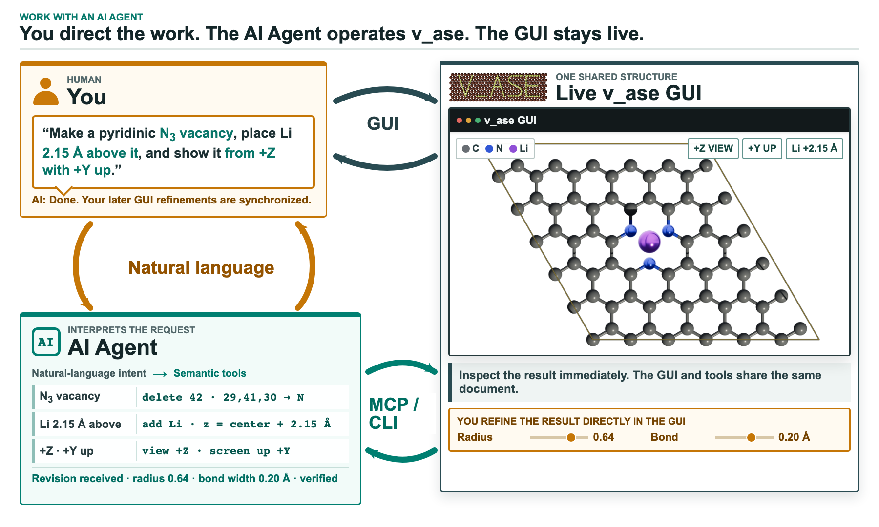
- You → Agent: describe the source system, requested scientific change, and final camera in ordinary language.
- Agent → v_ase: the Agent uses the Skill and structured CLI/API to read, modify, validate, and render exact atom data.
- v_ase → you: the result appears in the same live GUI. A manual GUI edit becomes the next document revision seen by the Agent.
v_ase does not interpret the natural-language request or embed an LLM. The external Agent translates it into exact, structured CLI/API operations.
For example, a human can ask:
From pristine 6 × 6 graphene, create a pyridinic N3 vacancy, place Li 2.15 Å above it, and render a +Z top view with +Y up at 4K.
The Agent identifies atoms from structured state rather than estimating them
from screenshots, preserves the three substituted sites as N_pyridinic, and
labels the adsorbate Li_site. It sets the requested +Z view and +Y up
direction before rendering.
Reading structured atom state instead of repeatedly interpreting screenshots
can reduce token use while keeping coordinates, labels, and camera settings
directly verifiable.
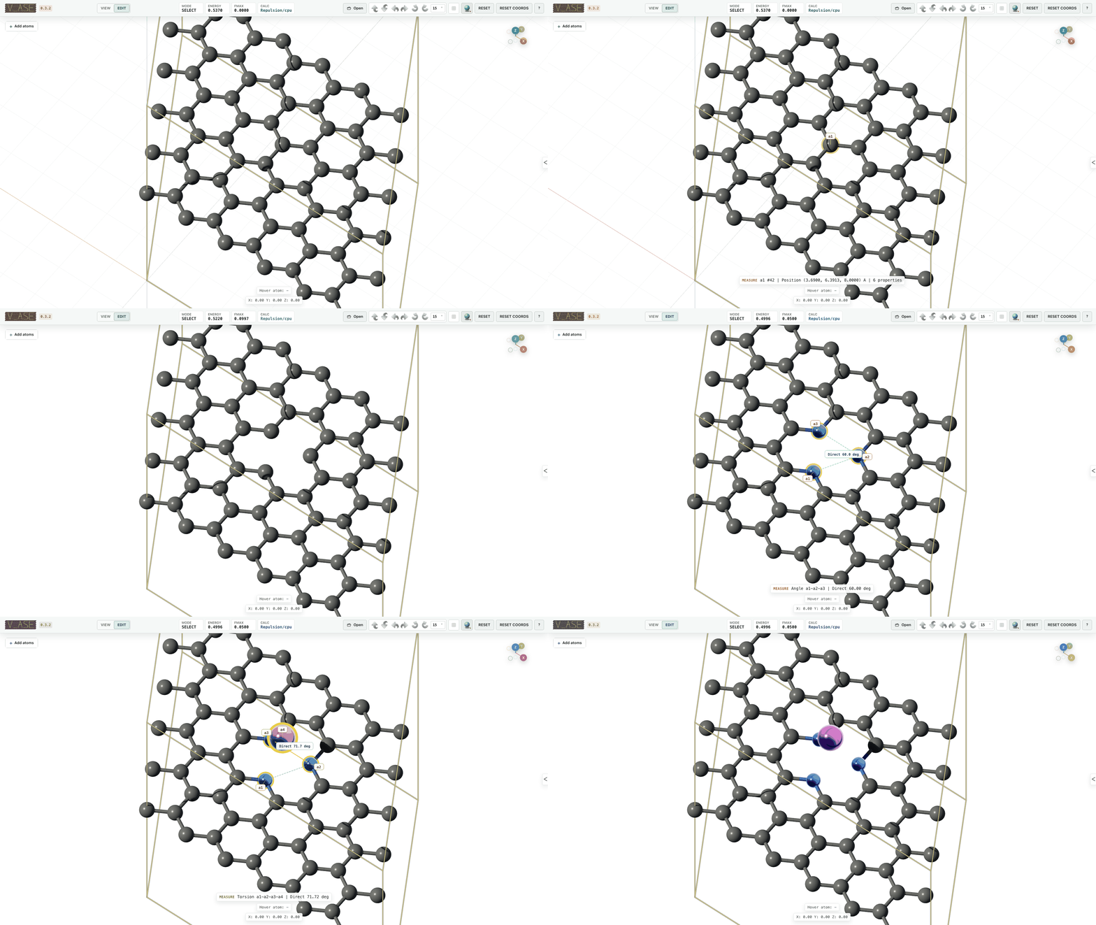
The example assets are generated from ase.build.graphene:
- source graphene CIF
- intermediate pyridinic N3 CIF
- final N3/Li-site CIF
- ASE trajectory preserving labels
Codex, Claude Code, and GitHub Copilot names and marks belong to their respective owners. They identify compatible external clients in the diagram; no affiliation or endorsement is implied.
Structure Manipulation
Use Edit when atom coordinates must change. Selection, measurement, appearance, bonds, replication, wrapping, visual translation, and export remain available in the default View mode.
Select
- Left-click selects one atom;
Shift+ click extends or removes selection. - Left-drag draws a visible selection box.
- Appearance rows select complete label groups without merging distinct labels.
- Ordered single-atom selections are retained for geometry measurement.
Move
Press G after selecting atoms. Lock the move with X, Y, or Z, type an
exact displacement in angstrom, then confirm with left-click or Enter.
Configured ASE constraints remain authoritative when Apply constraints is
enabled.
Rotate
Press R after selecting atoms. Choose Selection COM, Active atom (last
selected), Origin, or Unit-cell center as the pivot, lock an axis if
needed, and enter an exact angle. To rotate around a particular atom, select
the moving atoms first and Shift-select the pivot atom last. For a panel-driven
edit, use Structure > Transform > Exact selection rotation to choose the
axis and angle, then click Rotate Selection. Both methods honor the current
constraint and undo settings. Every active rotation shows:
- the rotation axis through the chosen pivot;
- a neutral line fixed at the direction where the operation started;
- an amber line that follows the current structure;
- cyan candidate lines only when the commensurate guide is enabled.
Ferrocene: Use Fe As The Active Pivot

Select the upper cyclopentadienyl ring first, then Shift-select Fe last. With Active atom (last selected) enabled, Fe remains fixed at the exact rotation pivot:
R,Zrotates the ring around the axis through Fe.R,Xfolds the same ring around an X axis through Fe.
The active atom can be any selected atom; it does not need to coincide with the global origin or the selection center.
Phosphorene: Build The Twist One Edit At A Time
The animation records a sequence of normal v_ase edits:
- Keep the first puckered ridge fixed. Left-drag the visible amber box from the second ridge through the end of the ribbon, then release to commit the yellow outlined selection.
- Open Structure > Transform, keep Selection COM, choose axis
X, enter1.538889degrees, and click Rotate Selection. - Close the panel, left-drag a new box from the third ridge through the end, enter the same exact angle, and rotate again from the edited coordinates.
- Continue advancing the box-selection boundary by one 12-atom ridge. After 9 rotations, the final ridge is rotated by exactly 13.85 degrees.
- Orbit the completed structure from above to below to inspect the full three-dimensional twist.
The amber box shows the current selection area, the yellow outline identifies the atoms affected by the next edit, and bonds update after each rotation.
Black phosphorene has two puckered sublayers in one armchair unit cell. The
5 x 6 model contains 10 puckered ridges with 12 atoms per ridge. Green and
purple distinguish the upper and lower P sublayers; both remain phosphorus in
the ASE structure.
The relaxed source coordinates come from the supporting information of Villegas et al.. The 13.85 degree target is one of the H-APNR angles tabulated by Jang et al., and the green/purple sublayer convention follows published phosphorene structure diagrams such as Zhang et al.. The example demonstrates geometry editing and is not an energy-minimized final structure.
Commensurate Atoms: Match Periodic 2D Cells
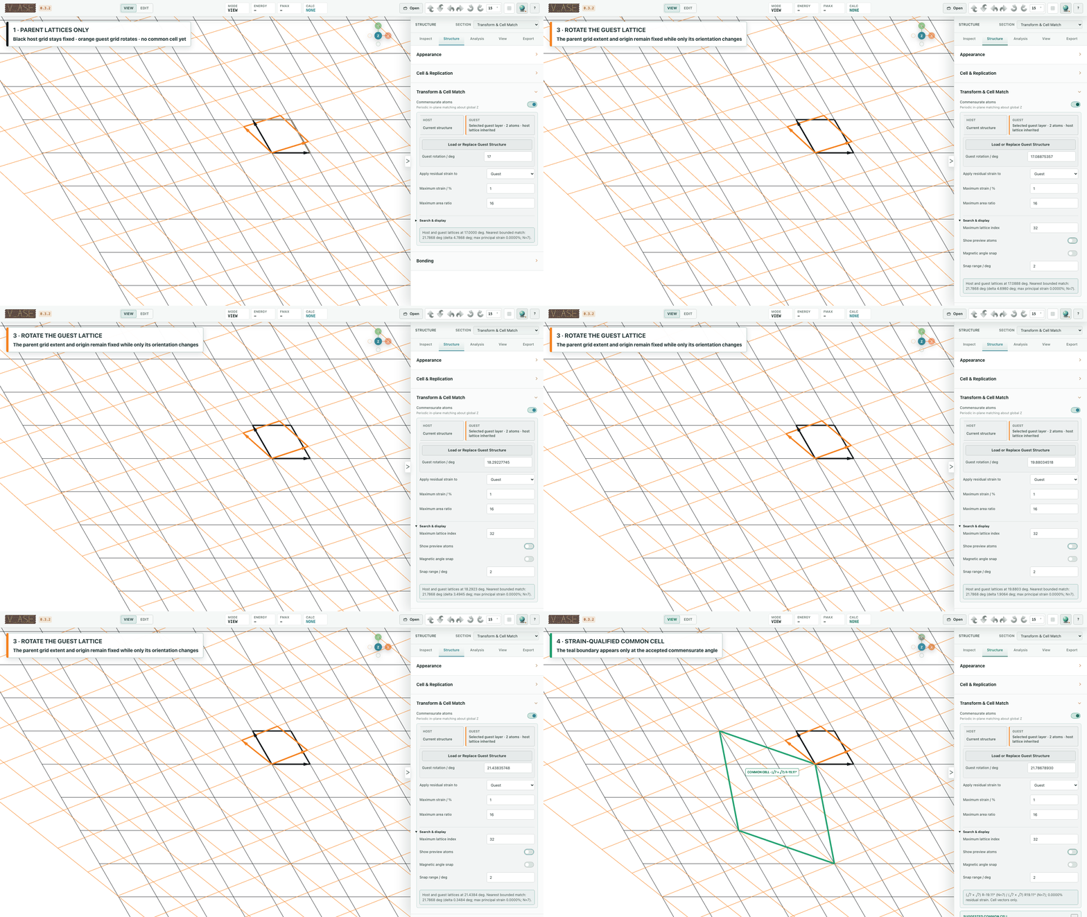
Commensurate atoms finds periodic in-plane common cells without changing the ASE structure until a proposal is explicitly accepted. It is off by default. When enabled, the first preview is cells-only:
- with no selected atoms, only the host primitive cell and vectors are shown;
- with a selected layer, those atoms become the guest and inherit a separate copy of the host cell;
- loading a guest structure replaces the selected guest with its own atoms and periodic cell.
Host primitive cells and vectors are black on the default white background, guest cells are orange, and the suggested common-cell boundary is teal. As a candidate or guest angle changes, both primitive lattices remain tiled through their proposed supercells in real time. The current camera is preserved. Show preview atoms optionally adds opaque supercell atoms, a one-primitive-cell halo, and all enabled bonds across the preview boundary.
The bounded search reports progress and opens an interactive graph:
| Graph | Meaning |
|---|---|
| Angle × cell size × strain | Rotation is the explicit horizontal axis; common-cell area forms depth layers and maximum principal strain is vertical; a live plane follows the current angle |
| Paper strain projection | Mean absolute strain versus the actual host-plus-guest atom count, with angle shown by color |
The graph's save icon exports the plotted angle, strain, host/guest integer
matrices, atom counts, surface notation, and method citations as CSV.
Maximum strain always uses the conservative maximum principal stretch;
switching graphs does not change accepted candidates. Maximum area ratio
defaults to 16 and is explicitly bounded at 128 so the interactive search
remains exhaustive instead of silently sampling a larger space.
Two workflows use the same bounded integer-boundary search:
| Workflow | Host | Guest / rotating component |
|---|---|---|
| Same-lattice twist | Unselected atoms and the current periodic cell | Selected atoms using a separate copy of that cell |
| Host/guest interface | The open structure and its cell | A second structure loaded with Load or Replace Guest Structure |
For a same-lattice graphene/hBN twist, select the hBN layer before enabling the
workspace. For a separate interface, load the guest file after enabling it.
The loaded guest is positioned so guest min z − host max z = 3 Å by default;
the Interlayer gap / Å field changes that separation. v_ase rotates the guest
atoms and guest cell together and never substitutes the host cell. Apply
residual strain to chooses whether the host or guest receives the remaining
in-plane deformation and defaults to the guest.
The proposal reports both integer matrices, both area ratios, residual strain,
and readable surface notation such as (√7 × √7) R19.11°. The default maximum
area ratio is 16. On first selection or guest load, v_ase proposes the
smallest-area cell that satisfies the strain bound. Moving the guest angle then
tracks the valid candidate nearest that angle. No proposal is made when every
valid cell exceeds the chosen area or strain bound.
Commensurate matching is deliberately restricted to two periodic vectors in the global XY plane and rotation about global Z. This is the rigorously defined 2D interface workflow; ordinary free atom rotation remains available when the workspace is off. Set Suggested Cell as Structure materializes the current validated proposal only in Edit mode. Trajectories and active volumetric fields remain preview-only because applying one inferred layer-specific cell to every frame or sampled field would be ambiguous.
The boundary-matching method follows the published integer-supercell and minimal-strain formulations in CellMatch and the optimal interface-supercell method. A full same-lattice hexagonal regression follows the commensurate integer-cell family in the twisted-bilayer graphene geometry. A suggested cell is a geometric periodic match, not an electronic energy minimum.
Separate Host And Guest Example
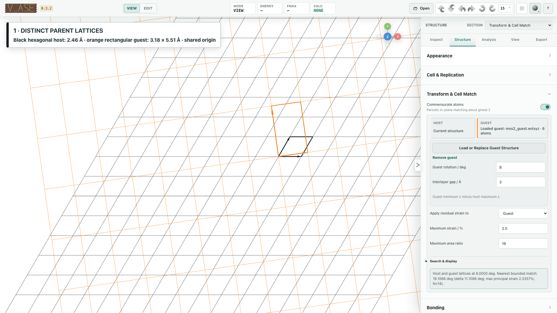
The repository includes a deterministic graphene/Cu(111) validation pair:
v_ase gui examples/commensurate_host_guest/graphene_host.extxyz
Enable Structure > Transform > Commensurate atoms, then load
cu111_guest.extxyz
with Load or Replace Guest Structure. Keep guest strain 1%, interlayer gap
3 Å, and maximum area ratio 16. The smallest match is graphene √13
against Cu(111) √12 at |16.10211375|°.
The common cell contains 26 graphene atoms plus 12 Cu atoms. The
example guide and
expected.json give the
exact maximum-principal and paper-style mean-strain values used by the tests.
The equations, numerical references, basis-invariance check, and measured search bounds are collected in Commensurate Cell Scientific Validation.
Normal R rotates selected atoms. Cell Transform is a separate periodic
operation that applies an integer matrix to the cell and every trajectory
frame. Display replication is separate again: it only repeats what is shown.
The common-cell equations, limits, and assumptions are documented in
unit_cell_aware_rotate.md.
Measurement And Analysis
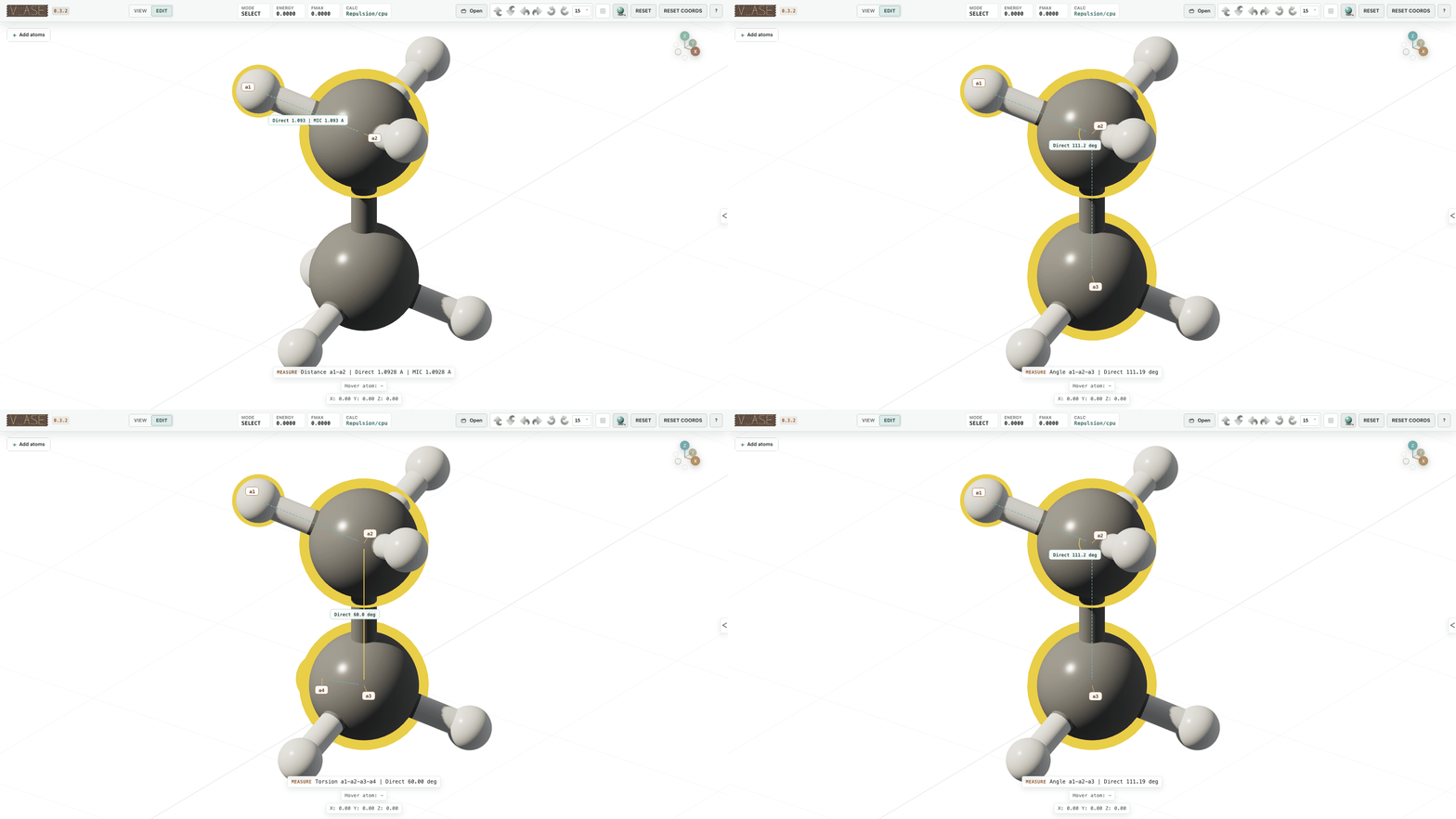
The numbered a1 to a4 markers record selection order and are deliberately
different from atom indices.
| Ordered selection | Reported result |
|---|---|
| 1 atom | Label, element, position, force, charge, tag, magnetic moment |
| 2 atoms | Direct distance and minimum-image distance |
| 3 atoms | Angle a1-a2-a3, centered on a2 |
| 4 atoms | Signed torsion a1-a2-a3-a4 |
| 5 or more | Total count and per-label counts |
The connector, angle arc, torsion axis, and compact value badge stay attached to the selected atoms. Hover information is independent, so moving the pointer does not replace a saved measurement.
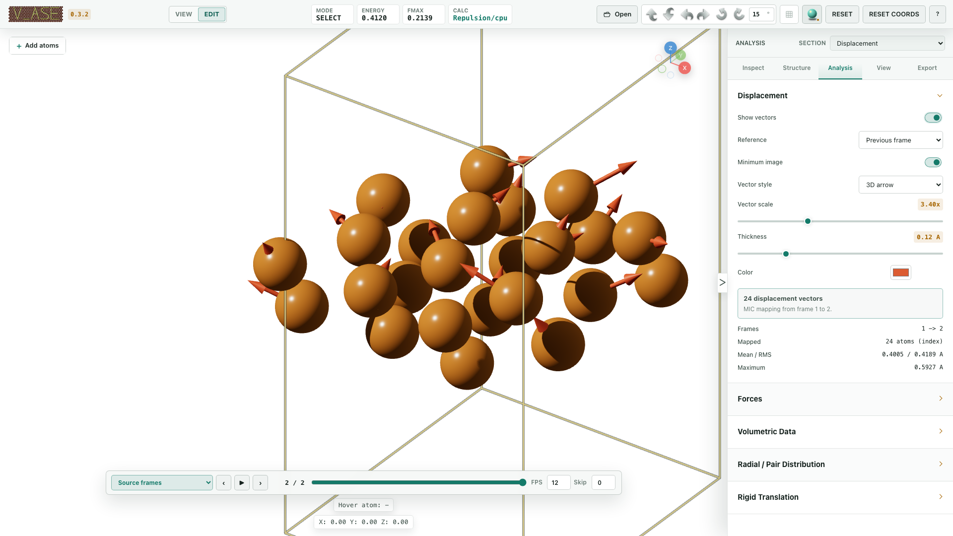
For trajectories, Analysis > Displacement compares the current frame with the previous frame or a chosen reference. Minimum-image correction, vector scale, thickness, color, and 2D/3D style are configurable. Displayed supercells repeat the vectors, and visual translation moves both endpoints without changing the physical displacement.
XY Registry Map
After choosing a periodic interface cell, select the layer or adsorbate that should translate and open Analysis > XY Registry Map. Starting the analysis without a selection produces a direct selection warning. v_ase scans one full periodic XY cell on the requested fractional grid while a staged progress display reports the active step.
The default Short-contact score is a dimensionless, covalent-radius-scaled geometry proxy. Bond-strain RMS instead uses enabled interfacial pairwise bond cutoffs and reports normalized bond-length mismatch for those pairs. Both scores are lower-is-better geometric screening metrics, not energies. Validate the proposed registry with an appropriate electronic-structure or force-field calculation before drawing physical conclusions.
The Plotly heatmap marks the best grid point and the current translation. While
the map is active, G is constrained to the periodic XY plane and the marker
follows the move continuously in fractional coordinates. The graph's save icon
exports the complete fractional X/Y grid, metric values, selected indices, and
method notes as CSV. RDF, commensurate, and registry plots all expose the same
adjacent save icon.
Volumetric Fields
Open a VASP CHGCAR, CHG, PARCHG, LOCPOT, or ELFCAR directly. Quantum
ESPRESSO and other electronic-structure codes can use Gaussian Cube or XSF
grid output:
v_ase gui CHGCAR
v_ase gui LOCPOT
v_ase gui charge-density.cube
v_ase gui charge-density.xsf
Analysis > Volumetric Data controls the dataset, isovalue, signed
positive/negative surfaces, mesh detail, field smearing, mesh smoothing,
colors, and isosurface opacity.
Opening a volumetric file, or adding the first scalar field, immediately shows
an isosurface at a valid default level. Drag Isosurface opacity to update
the current surface live without regenerating its mesh. Multiple compatible
datasets can be combined with coefficients such as +1, -1, -1 for a
charge-density difference. Grid values stay in the local v_ase backend; the
browser receives only the generated surface mesh.
Signed mode treats the isovalue as a nonzero magnitude and renders the
positive and negative crossings that remain inside the displayed field range.
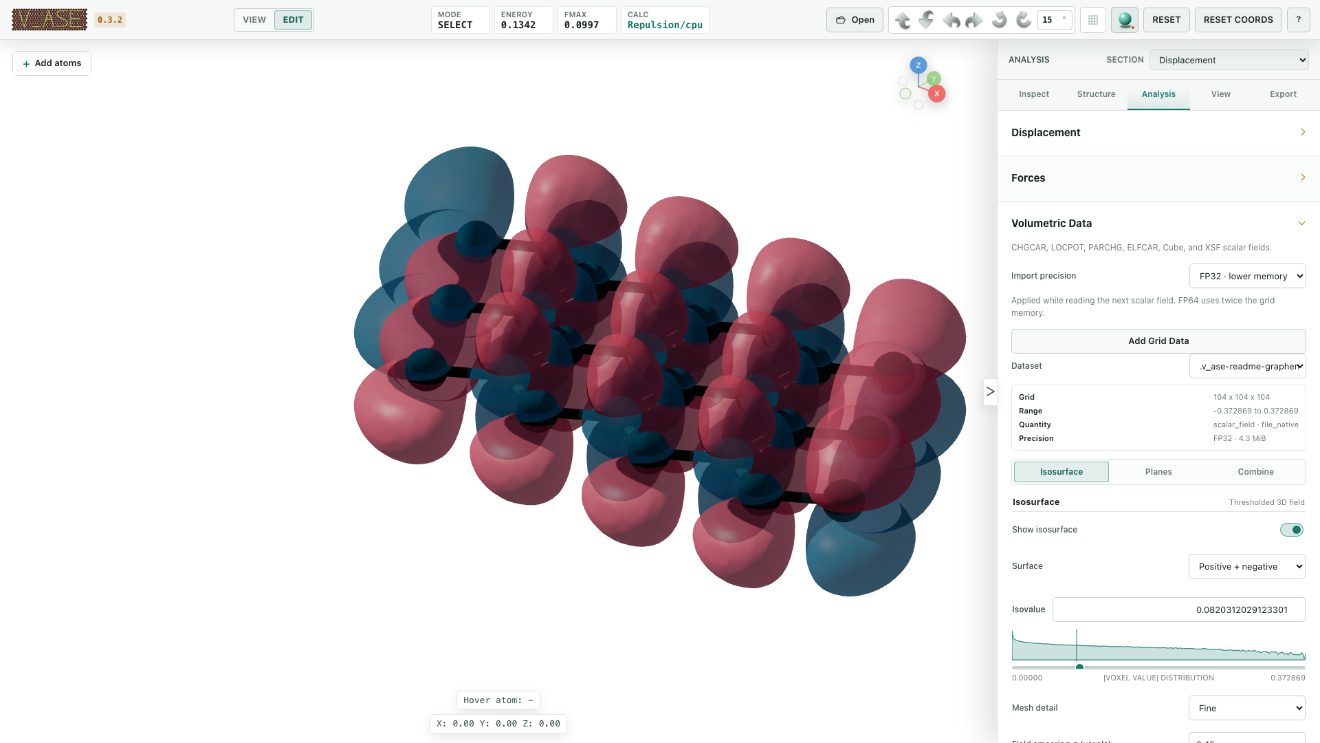
Field smearing σ applies a Gaussian filter measured in grid voxels before
the isosurface is extracted. Periodic directions wrap across the cell;
nonperiodic directions reflect at their boundary. Mesh smoothing passes
then reduce voxel stair-steps on the extracted mesh while keeping cell-boundary
vertices fixed. The source scalar field, its saved precision, integral, and
charge-density-difference inputs are never modified. Set either control to
0 to disable that stage. Because field smearing can merge small features or
change the range crossed by an isovalue, use the smallest value that removes
visible grid artifacts and verify the resulting topology.
Choose the import precision before opening or adding a scalar field. FP32 is the lower-memory default; FP64 preserves double-precision grid values and uses twice the grid memory. The same choice is available from the CLI:
v_ase gui CHGCAR --volumetric-precision fp64
The Python API exposes the same choice:
from v_ase.visualize import view

view("CHGCAR", volumetric_precision="fp64")
Visual translation and displayed cell replication move or repeat the isosurface together with the atoms. Set Supercell as Cell repeats both the ASE structure and periodic scalar grid exactly for diagonal integer replications. A general non-diagonal cell matrix is rejected while scalar grids are loaded because preserving that sampled field would require an explicit interpolation choice. After a materialized diagonal supercell, Reset Coordinates restores the original atoms, cell, and scalar grid together; Undo/Redo keeps the same atomic field pairing.
Radial Distribution Function
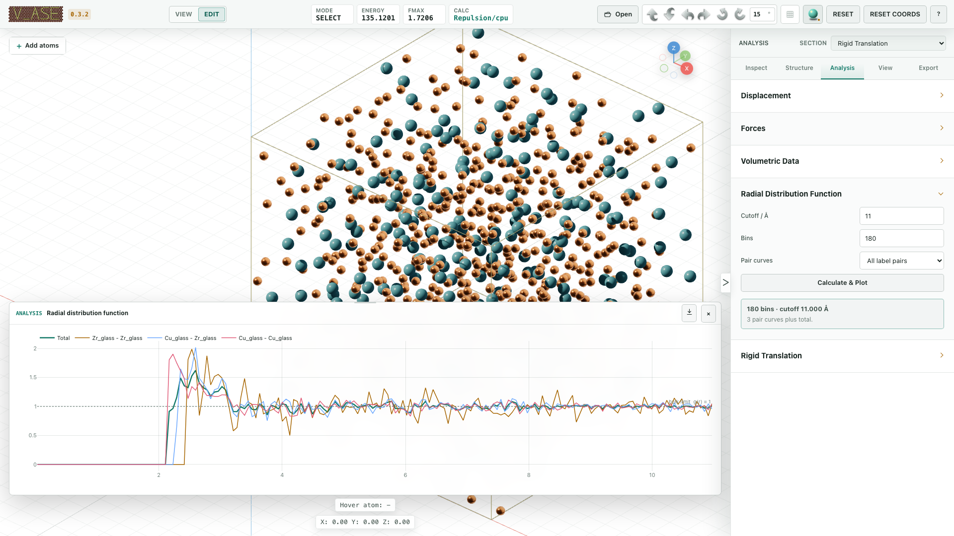
Analysis > Radial Distribution Function plots the current frame in a resizable Plotly drawer below the viewport. The total RDF is always included. Pair curves default to the active bond-label pairs and can be switched to all label pairs or total-only. Set the bin count and cutoff, then export exactly the plotted columns as CSV.
RDF uses exact spherical shell volumes and ASE's periodic neighbor search in
the full triclinic cell. The requested cutoff is not limited to a 2 x 2 x 2
replica or reduced at the unique minimum-image radius: v_ase includes every
periodic image whose distance falls inside the sphere and reports the image
span used. Bulk normalization is reported only for cells periodic in all three
directions; partial-PBC and finite systems require a separate boundary
correction and are rejected instead of returning a misleading bulk g(r).
The dotted g(r) = 1 reference makes the bulk limit explicit. In the
amorphous Cu-Zr example below, the broad short-range peak decays into a flat
long-range plateau rather than falling with the finite display cell.
Constraints
ASE remains authoritative when Apply constraints is enabled. Constraint visualization is local to each atom rather than merged at a group center.
FixedLine
A short cyan line passes through each constrained atom and remains visible
without selection. Starting G displays a longer guide through the atom's
original position while ASE restricts movement to that direction. FixedLine
does not use a ring or plane disc.

v_ase gui examples/readme_scene_assets/fixedline.traj --interactive
FixedPlane And FixScaled
Each constrained atom keeps its own local ring, crosshair, and normal marker.
When G starts, a larger translucent guide plane appears at that atom's
original position so the permitted surface remains visible while the atom
moves. Multiple selected atoms retain independent planes; no center-of-mass
plane is substituted.
VASP selective dynamics read as FixScaled are displayed from their allowed
fractional directions.

v_ase gui examples/readme_scene_assets/fixedplane.traj --interactive
FixAtoms
Fixed atoms keep their element color but use a distinct constrained surface treatment. They remain identifiable without looking selected.
Hookean
Hookean constraints show their inactive cutoff and engaged state separately.
After the constrained distance passes rt, a shaded 3D helical spring appears
between the constrained atoms.
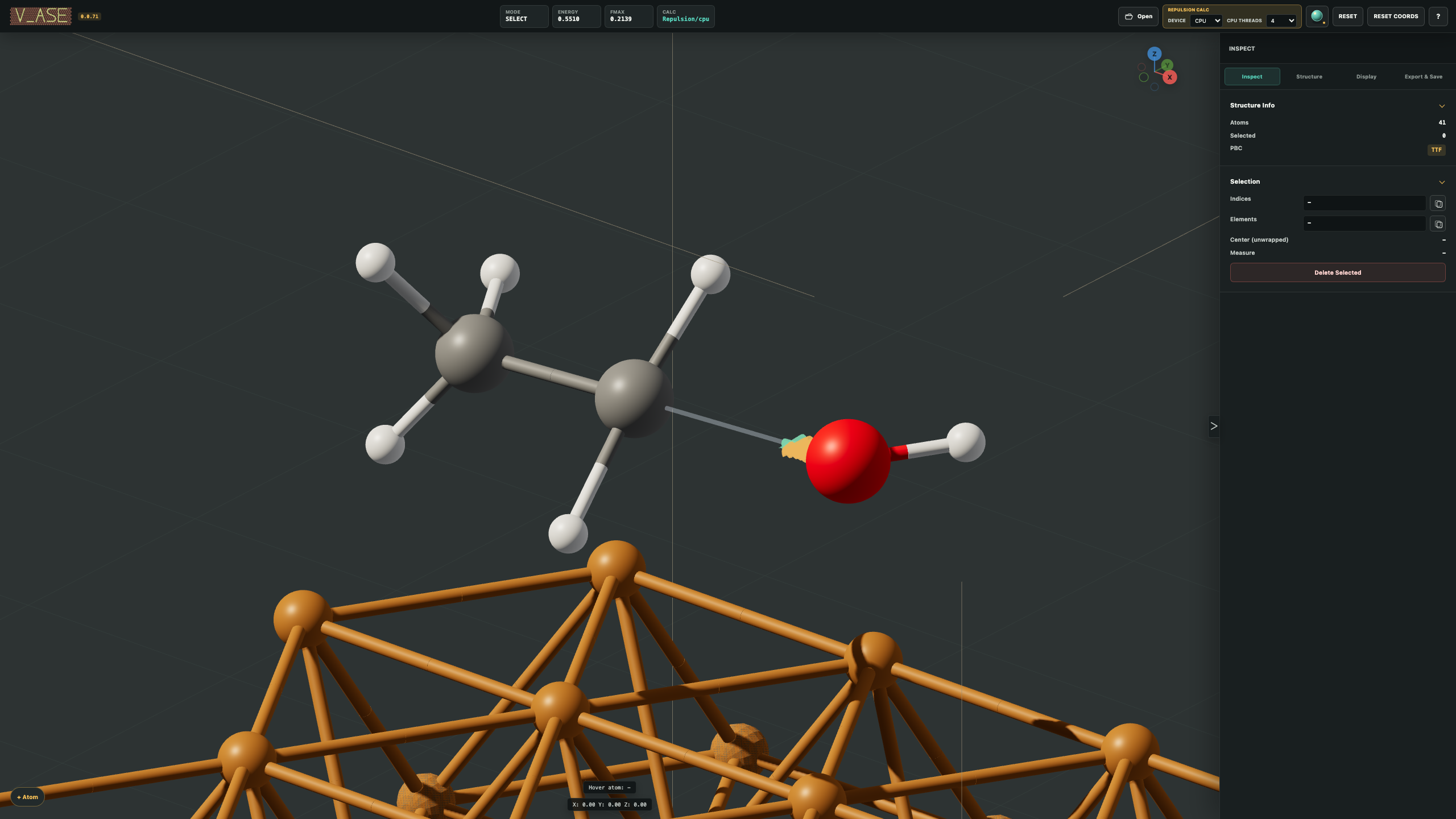

v_ase gui examples/readme_scene_assets/hookean.traj --interactive
Relaxation

Structure > Relaxation places every optimization step on a dedicated timeline. A single loaded structure gains a relaxation movie after the first run. If a source trajectory is already open, source and relaxation timelines remain separate and the active timeline is clearly selected.
The included example starts from a deliberately compressed C60 geometry and runs ASE FIRE with v_ase's repulsive fallback calculator:
v_ase gui examples/readme_scene_assets/crowded_c60_initial.cif --interactive
The fallback calculator is intended for removing obvious close contacts, not for predictive chemistry. Its cutoff scale and strength are editable. Attach a scientific ASE calculator when the optimized energy or forces will be used as physical results.
Trajectories
Multi-frame inputs add a timeline below the viewport. Scrubbing updates the
frame continuously, selected atom indices persist when topology permits, FPS
changes apply during playback, and Skip advances by skip + 1 source
frames per tick.
Bond topology is evaluated for each frame, so bonds form or break when a pair crosses its cutoff. Appearance, pair settings, supercell display, camera, and analysis settings remain active across the movie.
Video export uses FPS as playback speed. Optional N x interpolation creates
(source_frames - 1) * N + 1 output frames. Minimum-image interpolation uses
periodic cells to avoid jumps across a boundary. Interpolation takes longer
because more frames are rendered.
Appearance, Bonds, And Rendering
Structure > Appearance controls each stable atom label:
- ASE chemical TYPE and independent visual label;
- visibility and selection availability;
- color and radius;
- Standard, Metal, or Rubber material;
- all/partial/none selection checkbox.
View mode applies appearance by label. Edit mode can keep per-atom material overrides. Relabeling does not reorder the table or merge otherwise distinct atom types accidentally.
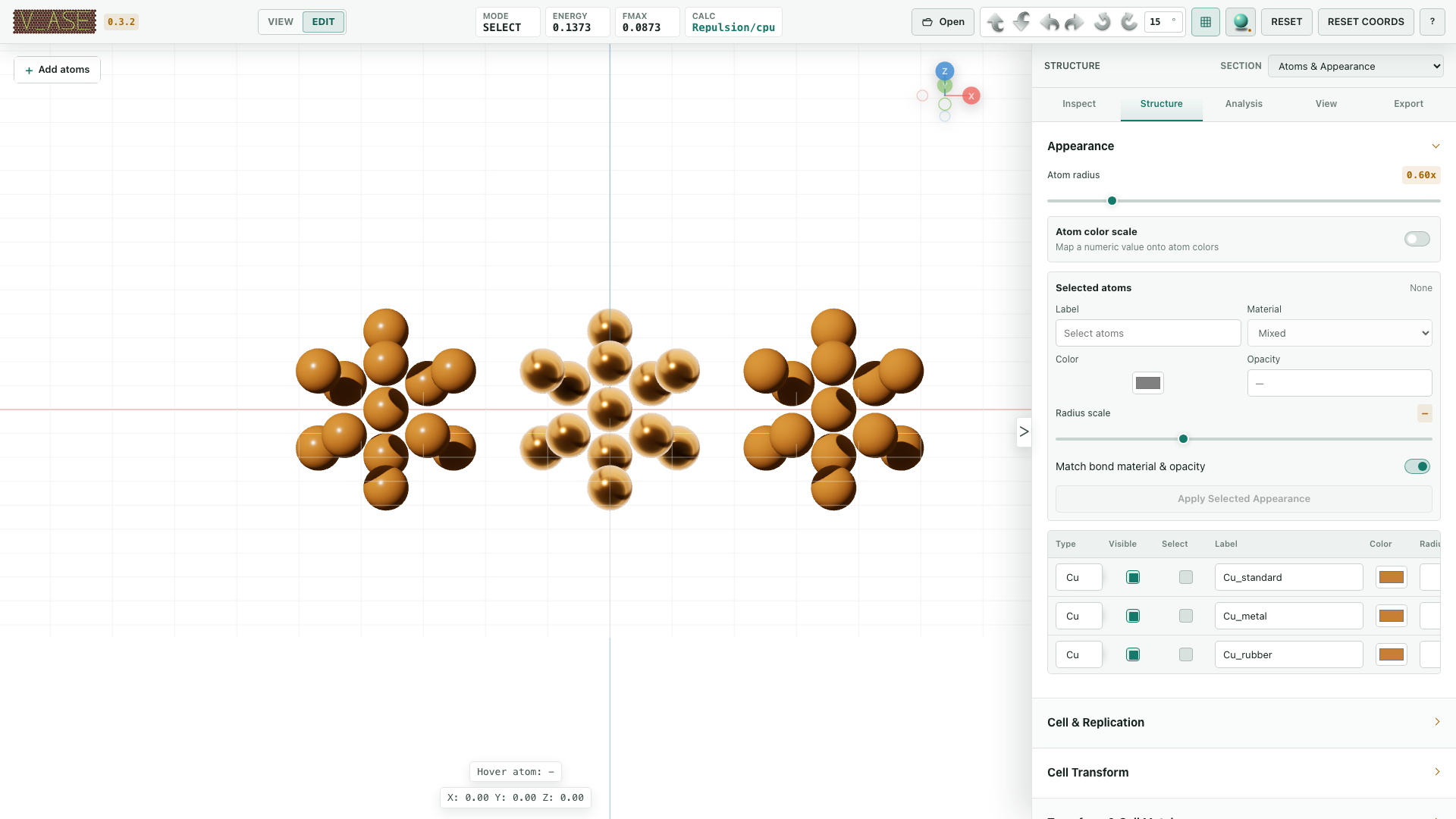
The comparison uses three identical Cu13 clusters with the same element color and radius, so only the optical material changes:
| Material | Visual response | Typical use |
|---|---|---|
| Standard | Balanced diffuse color and compact highlight | General structures and chemically neutral figures |
| Metal | Strong environment reflection and bright metallic highlight | Metals, electrodes, and reflective surfaces |
| Rubber | High roughness with broad, muted highlights | Soft visual grouping and low-glare nonmetal regions |
Materials affect rendering only. ASE elements, coordinates, calculators, and constraints are unchanged.
Atom colorscale maps a numeric per-atom property onto any registered Matplotlib colormap. The property list is discovered from the open structure and includes:
- Cartesian
x,y, andzcoordinates; - force magnitude when stored forces are available;
- scalar, component, and vector-norm views of numeric
Atoms.arraysvalues; - per-atom calculator results such as charge, magnetic moment, local energy, uncertainty, or model-specific MLIP outputs.
Use Selected atoms only to color the current selection while preserving
the established appearance of every other atom. Fit current frame is the
default range: it derives vmin and vmax once from the visible frame, then
keeps that range fixed while the trajectory plays. Scan trajectory finds a
single range across every frame without constructing a full in-memory value
cube. Entering either vmin or vmax switches to a manual range. Every frame
and export uses the resolved range consistently.
Reverse any map or adjust Contrast (gamma) from 0.1 to 5.0; gamma is
applied immediately in the browser without another scalar or colormap request.
The feature remains lazy: while its toggle is off, v_ase does not load a
colormap registry, extract scalar arrays, or run per-frame colorscale work.
Turning it off immediately restores the existing label, element, and per-atom
appearance.
Structure > Bonding provides automatic inference, explicit label-pair cutoffs, and manual index pairs. A pair cutoff of zero disables that pair. Changes apply immediately. Bonds support:
- cell-local or periodic minimum-image display;
- cylinder or flat 2D geometry;
- custom color or two half-bonds using the atom colors;
- configurable diameter;
- live formation and breaking during Edit transforms.
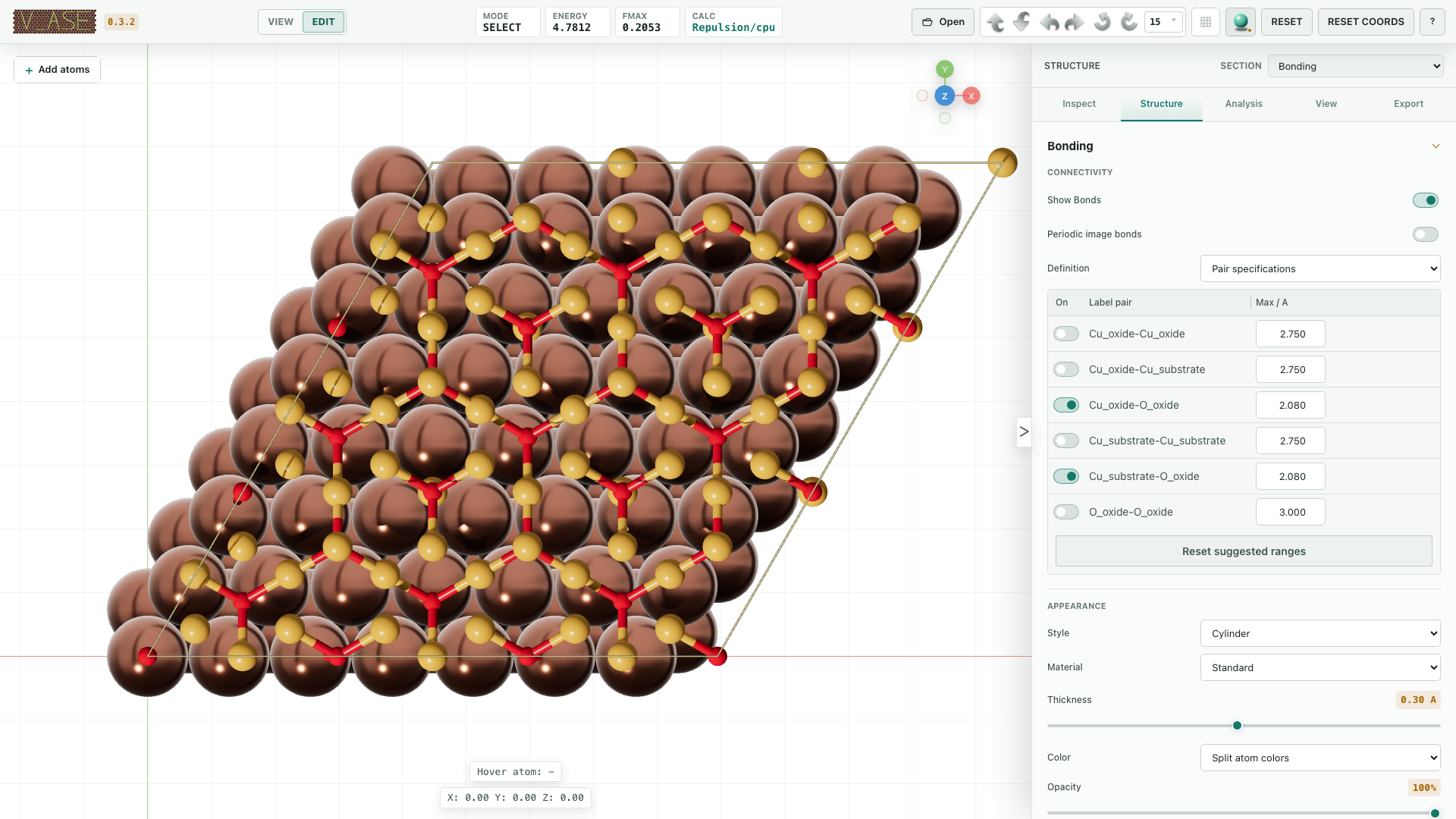
The top view shows a 6 x 6 Cu2O(111) film on 7 x 7 Cu(111), with one
interfacial oxygen positioned over a substrate Cu top site.
The Cu(111) substrate uses a nearest-neighbor touching-sphere radius.
Cu_oxide-O_oxide and Cu_substrate-O_oxide bonds are enabled, while
Cu_substrate-Cu_substrate, Cu_oxide-Cu_oxide, cross-region Cu-Cu, and
O-O pairs are disabled. Dark metallic substrate Cu, bright standard-material
oxide Cu, and matte red oxide O separate the phases without changing ASE
elements. Each bond is split into the colors of its two endpoint atoms, so the
Cu-O connectivity remains readable without an unrelated custom bond color.
Separate oxide and substrate labels let each interaction be enabled or
assigned its own cutoff independently.
v_ase gui examples/readme_scene_assets/cu2o111_on_cu111_pairwise_bonds.traj
View controls projection, atomic scale, anti-aliasing, sphere smoothness, background, 2D/3D display, grid, axes, unit cell, overlays, and cell material. The Axes and Unit Cell switches update the working viewport immediately; they are not export-only settings. Hiding world axes does not remove the compact orientation gizmo. New documents use orthographic projection and a true-white background.
The top-bar renderer switches between fast modeling light and Sun/soft-shadow rendering. Sun source, target, intensity, and direction can be manipulated in the viewport and carried into Blender export.
Interface Theme And Personal Defaults
View > Interface theme controls the application chrome independently from the white/dark 3D viewport background. System is the default and follows the browser or operating-system light/dark preference, including changes made while v_ase is open. Light and Dark keep an explicit choice in that browser.
Under Export > Visual Settings, Set Current as Default stores the current reusable appearance, bonds, lighting, viewport, display replication, visual translation, and render-quality choices for the current OS user. New structures and new tabs start with that style. Atom coordinates, trajectory frames, cell contents, absolute camera placement, and per-atom appearance overrides are not included.
Restore App Defaults deletes the saved personal default and applies the built-in v_ase style to the active tab. v_ase lists what will change and waits for Proceed; the structure itself is left untouched. Export Preset and Import Preset remain the portable file-based option for moving a visual preset between users or computers.
Export And Save
| Command | Result |
|---|---|
| Export POSCAR | Current physical ASE structure in VASP format |
| Export ASE Pickle | ASE Atoms, labels, constraints, arrays, and a valid SinglePointCalculator |
| Export Image | PNG by default; JPEG, PDF, and lossless WebP from the exact preview frame |
| Export Video | Constant-frame-rate H.264 MOV or MPEG-4 AVI with optional interpolation |
| Export Blender | Optimized scene script with atoms, bonds, cell, camera, and Sun |
| Export 3DM | Instanced Rhino geometry, metadata, and saved camera views |
| Export OBJ | OBJ/MTL, camera, and metadata in a ZIP |
| Export HTML View | Offline, view-only 3D document; lightweight by default, with optional .vase recovery |
Save .vase |
Compact project with structure/trajectory and complete visual state |
| HTML Project | Browser-ready project with complete embedded .vase recovery by default |
| Export/Import Preset | Portable visual settings file without coordinates |
Image, video, and HTML use one shared Preview Area composition. Its aspect ratio, camera, crop, lighting, atom scale, and included overlays match the saved output. HTML View defaults to grid off, axes on, and unit cell on; all three overlays can be changed before saving.
The system save picker is opened before expensive rendering or scene generation when the browser supports it. Canceling the picker cancels the export. Chrome may then show This site can view changes you make to this file. That message is Chrome's File System Access permission notice: v_ase can write only to the destination selected in that picker. Browser code cannot hide the notice while retaining destination selection before rendering.
Image export uses one determinate progress bar for rendering, pixel capture,
upload, encoding, download, and the final file write. It reports estimated
remaining time and reaches 100% once, only after the destination is complete.
Video export follows the same monotonic rule across all frames and encoding.
Every source frame is retained exactly once at 1x; interpolation adds
in-between frames. Visible displacement vectors and other selected scene
overlays are recalculated for each rendered frame.
Project Or Shareable HTML
Under Export > v_ase Project, use Save .vase for the smallest complete project. It contains every loaded frame, coordinates, cells, PBC, labels, constraints, safe calculator results, camera, appearance, bonds, lighting, analysis, and export settings. It is self-contained and never references the original input file.
Use HTML Project or HTML View when the result should open directly in a browser. The save dialog shows the exact shared Preview Area crop and lets you choose grid, axes, and unit-cell visibility. Every generated HTML:
- opens offline without v_ase, Python, a server, or a CDN;
- restores the saved camera, viewport styling, bonds, constraint overlays, displacement vectors, supercell, visual translation, and trajectory;
- allows orbit, pan, zoom, frame stepping, and movie playback;
- exposes no atom, structure, appearance, or project editing controls.
HTML View leaves Embed editable .vase project off by default and creates
the smaller view-only handoff. HTML Project enables it by default and stores
the complete .vase inside the same HTML. Embedded documents expose
Download .vase, and either command restores the full editable project:
v_ase gui project.vase
v_ase gui project.html
With project embedding disabled, the file is smaller and remains a portable view-only document. It cannot be restored as an editable v_ase project. v_ase reports this explicitly if that lightweight HTML is opened as input.
The exported frame is stored as an automatically optimized high-resolution poster as well as an interactive 3D scene. The initial HTML surface contains only that exact Preview Area crop: no v_ase logo, header, decorative border, or page margin is included. This lets macOS Finder/Quick Look show the structure without executing WebGL. In a browser, the first prepared WebGL frame replaces the poster with a short cross-fade as soon as the first live frame is ready, before camera input begins. Both surfaces occupy the same rectangle, so the structure does not jump. View-only controls appear only after pointer or keyboard activity.
HTML width and height inherit the image/video Preview Area. They define the saved camera aspect and crop, not a fixed live WebGL resolution. The interactive renderer automatically follows the browser size and display pixel density.
HTML is larger than .vase because it contains the browser renderer and
immediately readable scene data. Embedding adds a Base64 copy of .vase on
top of that. Keep .vase as the compact editable source of truth.
Opening an ordinary structure in an existing tab keeps the current visual
settings; opening .vase or project-embedded HTML restores the saved project.
Rhino export requires the optional dependency:
python -m pip install "v_ase-gui[rhino]"
OBJ export has no optional Python dependency.
Agent Setup
The AI agent runs separately from v_ase. Give it the complete v_ase Skill directory, then describe the result you want. The agent starts the machine-readable v_ase session, gives you the live GUI URL, and performs verified changes in that same document.
The Skill is vendor-neutral and can be used by Codex, Claude Code, ChatGPT desktop agents, Gemini-based agents, agentic IDEs, or another agent that can run local commands.
your natural-language request
  -> external AI agent + v_ase Skill
  -> v_ase structured CLI
  <-> the same live v_ase GUI you can watch and edit
--cli is not an embedded AI model. It is the structured connection the
external agent launches for itself. It exposes atomistic state and safe
operations, and reports committed GUI changes back to the agent. Revision
checks prevent an older agent command from silently replacing a newer human
edit.
What To Give The AI
Prefer the complete skill directory. If the client accepts only individual files, provide the following:
| Always provide | Add when the task needs it |
|---|---|
SKILL.md |
semantic-api.md for live state, edits, camera, render, or export |
agent-setup.md |
collaboration.md while a human and agent share the live GUI |
workflows-and-examples.md for multi-step scientific workflows |
|
cli-and-environments.md for installation, server, WSL, or process handling |
|
safety-and-errors.md before destructive edits, relaxation, or file output |
|
evaluation.md when changing or releasing v_ase itself |
For an AI client without a native skill loader, attach the files above and use:
Read SKILL.md and agent-setup.md. Use v_ase's structured CLI to inspect and
edit the structure, give me the live GUI URL so I can watch or refine it, honor
newer GUI changes before continuing, and verify both scientific state and the
final rendered output.
The compatibility document
skills_v_ase.md points existing integrations to the
same canonical skill and reference set.
Install The Skill
Clients with skill-folder support should install the complete directory:
# Codex
cp -R v_ase/skills/visualizing-atomic-structures-with-v-ase "$CODEX_HOME/skills/"

# Claude Code, from a project root
mkdir -p .claude/skills
cp -R v_ase/skills/visualizing-atomic-structures-with-v-ase .claude/skills/
For another AI, use its documented local skill directory if it supports the
same SKILL.md convention. Otherwise attach the files listed above or make
them readable in the project and include the bootstrap instruction.
Detailed CLI fields and command examples live in the Skill references rather than this user guide:
Documents And File Opening
The top-bar Open button starts with the operating system file picker. A selected file can:
- replace the active document;
- append structures to its current trajectory;
- open in a new independent v_ase tab.
If the active document is empty, the selected file opens there immediately; the destination chooser is shown only when a document already contains a structure or trajectory.
The + beside the document tabs creates an empty independent document. Each
tab owns its structure, trajectory, camera, selection, history, settings,
calculator, and .vase output.
Adding .vase to an existing trajectory imports only its structures and keeps
the current tab's visual state. Replacing a tab or opening a new one restores
the complete .vase project.
Python
from ase.build import molecule
from v_ase.visualize import view

atoms = molecule("H2O")
view(atoms)  # View mode
Inside Jupyter Notebook or JupyterLab, the same call automatically displays a view-only interactive model directly below the cell:
view(atoms)
The notebook output supports orbit, pan, zoom, and trajectory playback. After
importing view, use the %v_ase line magic to switch the default at any time:
%v_ase inline
view(atoms)  # interactive output below this cell

%v_ase browser
editor = view(atoms, block=False)  # full interface in an external browser

%v_ase auto  # restore automatic Jupyter detection
%load_ext v_ase.notebook registers the same magic explicitly when needed.
Passing notebook="inline" / True or notebook="browser" / False to one
view() call overrides the current magic setting.
When retaining an inline handle, display it explicitly:
from IPython.display import display

editor = view(atoms)
display(editor)
Return an edited ASE object:
edited = view(atoms, viz_only=False)
print(edited.positions)
view() accepts one ASE Atoms, a sequence of frames, or a supported file
path. view_edit() remains a compatibility alias for Edit mode.
File Formats
Common structure inputs include POSCAR/CONTCAR, VASP files, XDATCAR,
vasprun.xml, XYZ/extxyz, ASE .traj, LAMMPS dump/data, CIF, and .vase.
Volumetric inputs include VASP CHGCAR/CHG/PARCHG/LOCPOT/ELFCAR and Gaussian
Cube/XSF grids. ASE readers cover additional structure formats.
Use --format when an ambiguous filename does not identify the reader:
v_ase gui ABCD --format POSCAR
v_ase gui ABCD --format vasprun.xml
v_ase gui ABCD --format lammpstrj
v_ase gui ABCD --format data
v_ase gui ABCD --format CHGCAR
v_ase gui ABCD --format qe-cube
v_ase gui ABCD --format qe-xsf
Use --index : for every frame, --index -1 for the last frame, or an integer
for one frame.
Repeated POSCAR/CONTCAR species blocks remain separate visual labels. For
example, O Cu O with counts 1 14 5 becomes O1, Cu, and O2 while all
oxygen atoms remain ASE element O. Custom labels retain their complete text
when they are renamed or used for pair analysis.
Controls
| Input | Action |
|---|---|
| Left click / Shift + click | Select / extend selection |
| Left drag | Box select |
| Middle drag | Orbit without inertia |
| Shift + middle drag | Pan |
| Wheel | Zoom |
G / R |
Move / rotate selected atoms |
X, Y, Z during G/R |
Lock transform axis |
X, Y, Z otherwise |
Align camera to an axis |
| Number keys | Exact move distance or rotation angle |
Enter or left click |
Confirm transform |
Esc or right click |
Cancel transform |
Ctrl+C, Ctrl+V |
Copy and paste atoms |
Ctrl+Z, Ctrl+Shift+Z |
Undo and redo structure and visualization-setting changes; camera navigation is excluded |
Delete / Backspace |
Delete selected atoms |
Space |
Play or pause the active timeline |
| Left / Right Arrow | Previous / next frame in the active timeline |
Tab or Esc |
Open a collapsed control panel |
Esc with the panel open |
Close it and return focus to the viewport |
The ? button contains the complete shortcut table.
Remote Servers
Install v_ase on both the local computer and remote host, then run one command locally:
v_ase gui USER@SERVER:/absolute/path/to/STRUCTURE
An SSH config alias works:
v_ase gui physics:/absolute/path/to/trajectory.extxyz
v_ase selects private ports automatically, starts the backend beside the
remote file, creates the SSH tunnel, and opens the local browser. The source
file and full trajectory cache remain on the server; only the current frame
data required for local Three.js rendering crosses the tunnel. Use ProxyJump
in ~/.ssh/config when a login node is required.
License
v_ase releases from 0.1.11 onward are licensed under the
GNU Affero General Public License v3.0 or later
(AGPL-3.0-or-later). You may use,
modify, and redistribute the software under that license; distributions and
modified network services must satisfy its source-availability and
same-license requirements. Copyright (C) 2026 v_ase contributors.
The bundled Three.js module retains its own MIT license in
v_ase/static/vendor/THREE_LICENSE.
Troubleshooting
v_ase command is not found
Install and run with the same Python environment:
python -m pip install --upgrade v_ase-gui
python -m v_ase.cli --version
If the module command works but the console command does not, reactivate the
environment or add its Python scripts directory to PATH.
The browser does not open, or WSL prints gio: ... Operation not supported
The terminal also prints the complete local URL. Ctrl+click it or copy the text
beginning with http:// into Chrome, Edge, Firefox, or another browser. Keep
the terminal process running.
Example with sensitive session identifiers masked:
(base) giyeok@DESKTOP-XXXX:~$ v_ase gui
gio: http://127.0.0.1:58039/workspace?workspace_id=xxxx&session_id=xxxx: Operation not supported
For better WSL performance, keep trajectories under the Linux filesystem
rather than /mnt/c/....
A file is detected with the wrong format
Force the reader:
v_ase gui FILE --format POSCAR
v_ase gui FILE --format vasprun.xml
v_ase gui FILE --format lammpstrj
v_ase gui FILE --format data
Startup fails with cannot import name 'read_vasp_configuration'
This was an ASE 3.23/3.24 compatibility defect in v_ase 0.1.1 through 0.1.5. Upgrade v_ase in the same environment that provides the failing executable:
python -m pip install --upgrade "v_ase-gui>=0.1.6"
v_ase --version
v_ase 0.1.6 and later support the declared ase>=3.23 range without making
ordinary structure loading depend on a newer VASP-internal helper.
Replicated supercell atoms cannot be selected
In Edit, displayed replicas are noneditable previews. Use Set Supercell as Cell to create real ASE atoms and an editable larger cell. In View, displayed replicas are selectable and participate in center, distance, and other measurements.
Video export is unavailable or slow
Video export requires at least two frames and browser MediaRecorder support.
MOV/AVI conversion uses the bundled imageio-ffmpeg. Interpolation renders
additional frames and requires stable atom count, element, label, and ordering
between adjacent source frames. The selected FPS controls playback time:
72 frames at 30 FPS produce 2.40 seconds. The progress indicator reaches 100%
only after encoding and the destination write both finish.
Chrome says this site can view changes made to the saved file
This is a Chrome security notice for the File System Access API. v_ase opens the system save picker before a costly image, video, Blender, or 3D scene export so canceling does not waste time. It receives write access only to the file you choose. Chrome does not allow a page to suppress this notice; using an ordinary browser download would remove advance destination selection.
A large trajectory opens or plays slowly
- Keep the default View mode unless editing is required.
- Use
--stream-frameswhen frame data should be loaded on demand. - Keep browser hardware acceleration enabled.
- Close unused v_ase tabs; inactive tabs pause rendering but retain document state in memory.
- In WSL, keep data in the Linux filesystem.
RDF reports that fully periodic 3D boundaries are required
v_ase does not label a finite or partial-PBC histogram as a bulk RDF. Define a
valid 3D periodic cell for bulk g(r), or use a method with the boundary
correction appropriate to the finite, slab, or wire geometry.
Volumetric datasets cannot be combined
Density differences require identical grid dimensions, cell vectors, origin, PBC, endpoint convention, and units. Generate all component grids on the same FFT mesh, or resample them deliberately before opening them in v_ase.
Installation fails while pip checks an unrelated package version
A package version reported as None usually belongs to a different incomplete
or manually installed distribution in that environment. Run
python -m pip check, repair that distribution, or use a clean environment:
python -m venv .venv
python -m pip install --upgrade pip
python -m pip install v_ase-gui
Run v_ase --help or v_ase gui --help for all CLI options. Report
reproducible problems at
GitHub Issues.
1 maintainer

Download files
Download the file for your platform. If you're not sure which to choose, learn more about installing packages.
Source Distribution
Built Distribution
Filter files by name, interpreter, ABI, and platform.
If you're not sure about the file name format, learn more about wheel file names.
Copy a direct link to the current filters
File details
Details for the file v_ase_gui-0.1.14.tar.gz.
File metadata
- Download URL: v_ase_gui-0.1.14.tar.gz
- Upload date:
- Size: 7.6 MB
- Tags: Source
- Uploaded using Trusted Publishing? No
- Uploaded via:
twine/6.2.0 CPython/3.11.0
File hashes
| Algorithm | Hash digest | |
|---|---|---|
| SHA256 |
c6bdf92b895cf9d046482c2494ddfa16728789ca4bb5ba3ca5785e2d1bb31e2a
|
|
| MD5 |
c46561358c58adad0823f1dca4186f7b
|
|
| BLAKE2b-256 |
b30446b758b97474b0d8b025a81ca66df4f5659b516e93135a7817f4f8e57be9
|
File details
Details for the file v_ase_gui-0.1.14-py3-none-any.whl.
File metadata
- Download URL: v_ase_gui-0.1.14-py3-none-any.whl
- Upload date:
- Size: 7.4 MB
- Tags: Python 3
- Uploaded using Trusted Publishing? No
- Uploaded via:
twine/6.2.0 CPython/3.11.0
File hashes
| Algorithm | Hash digest | |
|---|---|---|
| SHA256 |
c8d54f1bf3313e24fc3faca3be64321938760b000ac529e1edb4490aa47fb59e
|
|
| MD5 |
4fff23c4aacafc8f71cefb4a2efb76ac
|
|
| BLAKE2b-256 |
ef36ff4da2f12e8b5f1f2c7a5b0bce62daf6a2614ab58a0e750d0ce843fb8e13
|














